Background
The relational model, developed as a result of recognized shortcomings
of hierarchical and network DBMSs, was introduced by Codd in 1970. As
the major developer, Codd believed that a sound theoretical model would
solve many practical problems that might arise.
In another article, Codd expounds the case for adopting the relational
over earlier database models. There is a threefold thrust to his
argument. First, earlier models forced the programmer to code at a
low level of structural detail. As a result, application programs are
more complex and took longer to write and debug. Second, no commands
were provided for processing multiple records at one time. Earlier models
did not provide the set-processing capability of the relational model.
The set-processing feature means that queries can be more concisely
expressed. Third, the relational model, through a query language such
as structured query language (SQL), recognizes the clients’ need to make
ad hoc queries. The relational model and SQL permit an IS department to
respond rapidly to unanticipated requests. It also meant that
analysts could write queries. Thus, Codd’s assertion that the
relational model is a practical tool for increasing the productivity of
IS departments is well founded.
The productivity increase arises from three of the objectives that drove
Codd’s research. The first was to provide a clearly delineated
boundary between the logical and physical aspects of database
management. Programming should be divorced from considerations of the
physical representation of data. Codd labels this the data
independence objective. The second objective was to create a simple
model that is readily understood by a wide range of analysts and
programmers. This communicability objective promotes effective and
efficient communication between clients and IS personnel. The third
objective was to increase processing capabilities from record-at-a-time
to multiple-records-at-a-time—the set-processing objective.
Achievement of these objectives means fewer lines of code are required
to write an application program, and there is less ambiguity in
client-analyst communication.
The relational model has three major components:
Data structures
Like most theories, the relational model is based on some key structures
or concepts. We need to understand these in order to understand the
theory.
Domain
A domain is a set of values all of the same data type. For example, the
domain of nation name is the set of all possible nation names. The
domain of all stock prices is the set of all currency values in, say,
the range $0 to $10,000,000. You can think of a domain as all the
legal values of an attribute.
In specifying a domain, you need to think about the smallest unit of
data for an attribute defined on that domain. In Chapter 8, we discussed
how a candidate attribute should be examined to see whether it should be
segmented (e.g., we divide name into first name, other name, and last
name, and maybe more). While it is unlikely that name will be a domain,
it is likely that there will be a domain for first name, last name, and
so on. Thus, a domain contains values that are in their atomic state;
they cannot be decomposed further.
The practical value of a domain is to define what comparisons are
permissible. Only attributes drawn from the same domain should be
compared; otherwise it is a bit like comparing bananas and strawberries.
For example, it makes no sense to compare a stock’s PE ratio to its
price. They do not measure the same thing; they belong to different
domains. Although the domain concept is useful, it is rarely supported
by relational model implementations.
Relations
A relation is a table of n columns (or attributes) and m rows (or
tuples). Each column has a unique name, and all the values in a column
are drawn from the same domain. Each row of the relation is uniquely
identified. The order of columns and rows is immaterial.
The cardinality of a relation is its number of rows. The degree
of a relation is the number of columns. For example, the relation nation
(see the following figure) is of degree 3 and has a cardinality of 4.
Because the cardinality of a relation changes every time a row is added
or deleted, you can expect cardinality to change frequently. The degree
changes if a column is added to a relation, but in terms of relational
theory, it is considered to be a new relation. So, only a relation’s
cardinality can change.
A relational database with tables nation and stock
| AUS |
Australia |
0.46 |
| IND |
India |
0.0228 |
| UK |
United Kingdom |
1 |
| USA |
United States |
0.67 |
| FC |
Freedonia Copper |
27.5 |
10,529 |
1.84 |
16 |
UK |
| PT |
Patagonian Tea |
55.25 |
12,635 |
2.5 |
10 |
UK |
| AR |
Abyssinian Ruby |
31.82 |
22,010 |
1.32 |
13 |
UK |
| SLG |
Sri Lankan Gold |
50.37 |
32,868 |
2.68 |
16 |
UK |
| ILZ |
Indian Lead & Zinc |
37.75 |
6,390 |
3 |
12 |
UK |
| BE |
Burmese Elephant |
0.07 |
154,713 |
0.01 |
3 |
UK |
| BS |
Bolivian Sheep |
12.75 |
231,678 |
1.78 |
11 |
UK |
| NG |
Nigerian Geese |
35 |
12,323 |
1.68 |
10 |
UK |
| CS |
Canadian Sugar |
52.78 |
4,716 |
2.5 |
15 |
UK |
| ROF |
Royal Ostrich Farms |
33.75 |
1,234,923 |
3 |
6 |
UK |
| MG |
Minnesota Gold |
53.87 |
816,122 |
1 |
25 |
USA |
| GP |
Georgia Peach |
2.35 |
387,333 |
0.2 |
5 |
USA |
| NE |
Narembeen Emu |
12.34 |
45,619 |
1 |
8 |
AUS |
| QD |
Queensland Diamond |
6.73 |
89,251 |
0.5 |
7 |
AUS |
| IR |
Indooroopilly Ruby |
15.92 |
56,147 |
0.5 |
20 |
AUS |
| BD |
Bombay Duck |
25.55 |
167,382 |
1 |
12 |
IN |
Relational database
A relational database is a collection of relations or tables. A
distinguishing feature of the relational model, is that there are no explicit linkages between tables. Tables are linked by common columns drawn on the same
domain; thus, the portfolio database (see the preceding tables) consists
of tables stock and nation. The 1:m relationship between the two
tables is represented by the column natcode that is common to both
tables. Note that the two columns need not have the same name, but they
must be drawn on the same domain so that comparison is possible. In the
case of an m:m relationship, while a new table must be created to
represent the relationship, the principle of linking tables through
common columns on the same domain remains in force.
Primary key
A relation’s primary key is its unique identifier; for example, the
primary key of nation is natcode. As you already know, a primary key
can be a composite of several columns. The primary key guarantees that
each row of a relation can be uniquely addressed.
Candidate key
In some situations, there may be several attributes, known as candidate
keys, that are potential primary keys. Column natcode is unique in the
nation relation, for example. We also can be fairly certain that two
nations will not have the same name. Therefore, nation has multiple
candidate keys: natcode and natname.
Alternate key
When there are multiple candidate keys, one is chosen as the primary
key, and the remainder are known as alternate keys. In this case, we
selected natcode as the primary key, and natname is an alternate
key.
Foreign key
The foreign key is an important concept of the relational model. It is
the way relationships are represented and can be thought of as the glue
that holds a set of tables together to form a relational database. A
foreign key is an attribute (possibly composite) of a relation that is
also a primary key of a relation. The foreign key and primary key may be
in different relations or the same relation, but both keys must be drawn
from the same domain.
Integrity rules
The integrity section of the relational model consists of two rules. The
entity integrity rule ensures that each instance of an entity
described by a relation is identifiable in some way. Its implementation
means that each row in a relation can be uniquely distinguished. The
rule is
No component of the primary key of a relation may be null.
Null in this case means that the component cannot be undefined or
unknown; it must have a value. Notice that the rule says “component of a
primary key.” This means every part of the primary key must be known. If
a portion of the key cannot be defined, it implies that the particular entity it
describes cannot be defined. In practical terms, it means you cannot add
a nation to nation unless you also define a value for natcode.
The definition of a foreign key implies that there is a corresponding
primary key. The referential integrity rule ensures that this is the
case. It states
A database must not contain any unmatched foreign key values.
Simply, this rule means that you cannot define a foreign key without
first defining its matching primary key. In practical terms, it would
mean you could not add a Canadian stock to the stock relation without
first creating a row in nation for Canada.
Notice that the concepts of foreign key and referential integrity are
intertwined. There is not much sense in having foreign keys without
having the referential integrity rule. Permitting a foreign key without
a corresponding primary key means the relationship cannot be determined.
Note that the referential integrity rule does not imply a foreign key
cannot be null. There can be circumstances where a relationship does not
exist for a particular instance, in which case the foreign key is null.
Manipulation languages
There are four approaches to manipulating relational tables, and you are
already familiar with SQL, the major method.
Query-by-example (QBE), which describes a
general class of graphical interfaces to a relational database to make
it easier to write queries, is also commonly used. Less widely used
manipulation languages are relational algebra and relational calculus.
These languages are briefly discussed, with some attention given to
relational algebra in the next section and SQL in the following chapter.
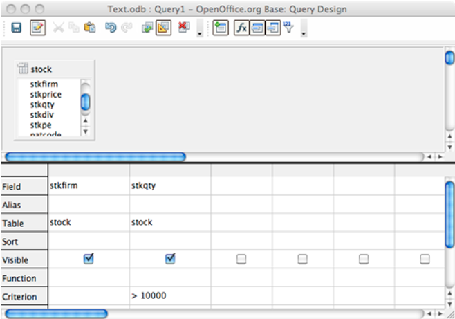
Query-by-example (QBE) is not a standard, and each vendor implements
the idea differently. The general principle is to enable those with
limited SQL skills to interrogate a relational database. Thus, the
analyst might select tables and columns using drag and drop or by
clicking a button. The following screen shot shows the QBE interface to
LibreOffice, which is very similar to that of MS Access. It shows
selection of the stock table and two of its columns, as well as a
criterion for stkqty. QBE commands are translated to SQL prior to
execution, and many systems allow you to view the generated SQL. This
can be handy. You can use QBE to generate a portion of the SQL for a
complex query and then edit the generated code to fine-tune the query.
Query-by-example with LibreOffice
Relational algebra has a set of operations similar to traditional
algebra (e.g., add and multiply) for manipulating tables. Although
relational algebra can be used to resolve queries, it is seldom
employed, because it requires you to specify both what you want and how
to get it. That is, you have to specify the operations on each table.
This makes relational algebra more difficult to use than SQL, where the
focus is on specifying what is wanted.
Relational calculus overcomes some of the shortcomings of relational
algebra by concentrating on what is required. In other words, there is
less need to specify how the query will operate. Relational calculus is
classified as a nonprocedural language, because you do not have to be
overly concerned with the procedures by which a result is determined.
Unfortunately, relational calculus can be difficult to learn, and as a
result, language designers developed SQL and QBE, which are
nonprocedural and more readily mastered. You have already gained some
skills in SQL. Although QBE is generally easier to use than SQL, IS
professionals need to master SQL for two reasons. First, SQL is
frequently embedded in other programming languages, a feature not
available with QBE. Second, it is very difficult, or impossible, to
express some queries in QBE (e.g., divide). Because SQL is important, it
is the focus of the next chapter.
Relational algebra
The relational model includes a set of operations, known as relational
algebra, for manipulating relations. Relational algebra is a standard
for judging data retrieval languages. If a retrieval language, such as
SQL, can be used to express every relational algebra operator, it is
said to be relationally complete.
Relational algebra operators
| Restrict |
Creates a new table from specified rows of an existing table |
| Project |
Creates a new table from specified columns of an existing table |
| Product |
Creates a new table from all the possible combinations of rows of two existing tables |
| Union |
Creates a new table containing rows appearing in one or both tables of two existing tables |
| Intersect |
Creates a new table containing rows appearing in both tables of two existing tables |
| Difference |
Creates a new table containing rows appearing in one table but not in the other of two existing tables |
| Join |
Creates a new table containing all possible combinations of rows of two existing tables satisfying the join condition |
| Divide |
Creates a new table containing xi such that the pair (xi, yi) exists in the first table for every yi in the second table |
There are eight relational algebra operations that can be used with
either one or two relations to create a new relation. The assignment
operator (:=) indicates the name of the new relation. The relational
algebra statement to create relation A, the union of relations B and C,
is expressed as
A := B UNION C
Before we begin our discussion of each of the eight operators, note that
the first two, restrict and project, operate on a single relation and
the rest require two relations.
Restrict
Restrict extracts specified rows from a single relation. It takes a horizontal slice through a relation.
Project
Project extracts specified columns from a table. It takes a vertical slice through a table.
Product
Product creates a new relation from all possible combinations of rows in
two other relations. It is sometimes called TIMES or MULTIPLY. The
relational command to create the product of two tables is
The operation of product is illustrated in the following figure, which
shows the result of A TIMES B.
Relational operator product
| V |
W |
|
X |
Y |
Z |
| v1 |
w1 |
|
x1 |
y1 |
z1 |
| v2 |
w2 |
|
x2 |
y2 |
z2 |
| v3 |
w3 |
|
|
|
|
A TIMES B
| v1 |
w1 |
x1 |
y1 |
z1 |
| v1 |
w1 |
x2 |
y2 |
z2 |
| v2 |
w2 |
x1 |
y1 |
z1 |
| v2 |
w2 |
x2 |
y2 |
z2 |
| v3 |
w3 |
x1 |
y1 |
z1 |
| v3 |
w3 |
x2 |
y2 |
z2 |
Union
The union of two relations is a new relation containing all rows
appearing in one or both relations. The two relations must be union
compatible, which means they have the same column names, in the same
order, and drawn on the same domains. Duplicate rows are automatically
eliminated—they must be, or the relational model is no longer
satisfied. The relational command to create the union of two tables is
Union is illustrated in the following figure. Notice that corresponding
columns in tables A and B have the same names. While the sum of the
number of rows in relations A and B is five, the union contains four
rows, because one row (x2, y2 ) is common to both relations.
Relational operator union
| X |
Y |
|
X |
Y |
| x1 |
y1 |
|
x2 |
y2 |
| x2 |
y2 |
|
x4 |
y4 |
| x3 |
y3 |
|
|
|
A UNION B
Intersect
The intersection of two relations is a new relation containing all rows
appearing in both relations. The two relations must be union compatible.
The relational command to create the intersection of two tables is
The result of A INTERSECT B is one row, because only one row (x2,
y2) is common to both relations A and B.
Relational operator intersect
| X |
Y |
|
X |
Y |
| x1 |
y1 |
|
x2 |
y2 |
| x2 |
y2 |
|
x4 |
y4 |
| x3 |
y3 |
|
|
|
A INTERSECT B
Difference
The difference between two relations is a new relation containing all
rows appearing in the first relation but not in the second. The two
relations must be union compatible. The relational command to
create the difference between two tables is
The result of A MINUS B is two rows (see the following figure). Both of
these rows are in relation A but not in relation B. The row containing
(x1, y2) appears in both A and B and thus is not in A MINUS B.
Relational operator difference
| X |
Y |
|
X |
Y |
| x1 |
y1 |
|
x2 |
y2 |
| x2 |
y2 |
|
x4 |
y4 |
| x3 |
y3 |
|
|
|
A MINUS B
Join
Join creates a new relation from two relations for all combinations of
rows satisfying the join condition. The general format of join is
where theta can be =, <>, >, >=, <, or <=.
The following figure illustrates A JOIN B WHERE W = Z, which is an
equijoin because theta is an equals sign. Tables A and B are matched
when values in columns W and Z in each relation are equal. The matching
columns should be drawn from the same domain. You can also think of join
as a product followed by restrict on the resulting relation.
Relational operator join
| V |
W |
|
X |
Y |
Z |
| v1 |
wz1 |
|
x1 |
y1 |
wz1 |
| v2 |
wz2 |
|
x2 |
y2 |
wz2 |
| v3 |
wz3 |
|
|
|
|
A EQUIJOIN B
| v1 |
wz1 |
x1 |
y1 |
wz1 |
| v3 |
wz3 |
x2 |
y2 |
wz3 |
Divide
Divide is the hardest relational operator to understand. Divide requires
that A and B have a set of attributes, in this case Y, that are common
to both relations. Conceptually, A divided by B asks the question, “Is
there a value in the X column of A (e.g., x1) that has a value in the
Y column of A for every value of y in the Y column of B?” Look first at
B, where the Y column has values y1 and y2. When you examine the X
column of A, you find there are rows (x1, y1) and (x1, y2). That
is, for x1, there is a value in the Y column of A for every value of y
in the Y column of B. Thus, the result of the division is a new relation
with a single row and column containing the value x1.
Relational operator divide
| X |
Y |
|
Y |
| x1 |
y1 |
|
y1 |
| x1 |
y3 |
|
y2 |
| x1 |
y2 |
|
|
| x2 |
y1 |
|
|
| x3 |
y3 |
|
|
A DIVIDE B
A primitive set of relational operators
The full set of eight relational operators is not required. As you have
already seen, join can be defined in terms of product and restrict.
Intersection and divide can also be defined in terms of other commands.
Indeed, only five operators are required: restrict, project, product,
union, and difference. These five are known as primitives because
these are the minimal set of relational operators. None of the primitive
operators can be defined in terms of the other operators.
A fully relational database
The three components of a relational database system are structures
(domains and relations), integrity rules (primary and foreign keys), and
a manipulation language (relational algebra). A fully relational
database system provides complete support for each of these
components. Many commercial systems support SQL but do not provide
support for domains. Such systems are not fully relational but are
relationally complete.
In 1985, Codd established the 12 commandments of relational database
systems (see the following table). In addition to providing some
insights into Codd’s thinking about the management of data, these rules
can also be used to judge how well a database fits the relational model.
The major impetus for these rules was uncertainty in the marketplace
about the meaning of “relational DBMS.” Codd’s rules are a checklist for
establishing the completeness of a relational DBMS. They also provide a
short summary of the major features of the relational DBMS.
Codd’s rules for a relational DBMS
| The information rule |
| The guaranteed access rule |
| Systematic treatment of null values |
| Active online catalog of the relational model |
| The comprehensive data sublanguage rule |
| The view updating rule |
| High-level insert, update, and delete |
| Physical data independence |
| Logical data independence |
| Integrity independence |
| Distribution independence |
| The nonsubversion rule |
The guaranteed access rule
Every value in a database must be addressable by specifying its table
name, column name, and the primary key of the row in which it is stored.
Systematic treatment of null values
There must be a distinct representation for unknown or inappropriate
data. This must be unique and independent of data type. The DBMS should
handle null data in a systematic way. For example, a zero or a blank
cannot be used to represent a null. This is one of the more troublesome
areas because null can have several meanings (e.g., missing or
inappropriate).
Active online catalog of the relational model
There should be an online catalog that describes the relational model.
Authorized users should be able to access this catalog using the DBMS’s
query language (e.g., SQL).
The comprehensive data sublanguage rule
There must be a relational language that supports data definition, data
manipulation, security and integrity constraints, and transaction
processing operations. Furthermore, this language must support both
interactive querying and application programming and be expressible in
text format. SQL fits these requirements.
The view updating rule
The DBMS must be able to update any view that is theoretically
updatable.
High-level insert, update, and delete
The system must support set-at-a-time operations. For example, multiple
rows must be updatable with a single command.
Physical data independence
Changes to storage representation or access methods will not affect
application programs. For example, application programs should remain
unimpaired even if a database is moved to a different storage device or
an index is created for a table.
Logical data independence
Information-preserving changes to base tables will not affect
application programs. For instance, no applications should be affected
when a new table is added to a database.
Integrity independence
Integrity constraints should be part of a database’s definition rather
than embedded within application programs. It must be possible to change
these constraints without affecting any existing application programs.
Distribution independence
Introduction of a distributed DBMS or redistribution of existing
distributed data should have no impact on existing applications.
The nonsubversion rule
It must not be possible to use a record-at-a-time interface to subvert
security or integrity constraints. You should not be able, for example,
to write a Java program with embedded SQL commands to bypass security
features.
Codd issued an additional higher-level rule, rule 0, which states that a
relational DBMS must be able to manage databases entirely through its
relational capacities. In other words, a DBMS is either totally
relational or it is not relational.
Summary
The relational model developed as a result of recognized shortcomings of
hierarchical and network DBMSs. Codd created a strong theoretical base
for the relational model. Three objectives drove relational database
research: data independence, communicability, and set processing. The
relational model has domain structures, integrity rules, and operators
used to retrieve, derive, or modify data. A domain is a set of values
all of the same data type. The practical value of a domain is to define
what comparisons are permissible. A relation is a table of n columns
and m rows. The cardinality of a relation is its number of rows. The
degree of a relation is the number of columns.
A relational database is a collection of relations. The distinguishing
feature of the relational model is that there are no explicit linkages
between tables. A relation’s primary key is its unique identifier. When
there are multiple candidates for the primary key, one is chosen as the
primary key and the remainder are known as alternate keys. The foreign
key is the way relationships are represented and can be thought of as
the glue that binds a set of tables together to form a relational
database. The purpose of the entity integrity rule is to ensure that
each entity described by a relation is identifiable in some way. The
referential integrity rule ensures that you cannot define a foreign key
without first defining its matching primary key.
The relational model includes a set of operations, known as relational
algebra, for manipulating relations. There are eight operations that can
be used with either one or two relations to create a new relation. These
operations are restrict, project, product, union, intersect, difference,
join, and divide. Only five operators, known as primitives, are required
to define all eight relational operations. An SQL statement can be
translated to relational algebra and vice versa. If a retrieval language
can be used to express every relational algebra operator, it is said to
be relationally complete. A fully relational database system provides
complete support for domains, integrity rules, and a manipulation
language. Codd set forth 12 rules that can be used to judge how well a
database fits the relational model. He also added rule 0—a DBMS is
either totally relational or it is not relational.
Key terms and concepts
| Alternate key |
Join |
| Candidate key |
Logical data independence |
| Cardinality |
Nonsubversion rule |
| Catalog |
Null |
| Communicability objective |
Operators |
| Data independence |
Physical data independence |
| Data structures |
Primary key |
| Data sublanguage rule |
Product |
| Degree |
Project |
| Difference |
Query-by-example (QBE) |
| Distribution independence |
Referential integrity |
| Divide |
Relational algebra |
| Domain |
Relational calculus |
| Entity integrity |
Set processing objective |
| Foreign key |
Relational database |
| Fully relational database |
Relational model |
| Guaranteed access rule |
Relationally complete |
| Information rule |
Relations |
| Integrity independence |
Restrict |
| Integrity rules |
Union |
| Intersect |
View updating rule |
References and additional readings
Codd, E. F. 1982. Relational database: A practical foundation for
productivity. Communications of the ACM 25 (2):109–117.