SQL
The questing beast.
Sir Thomas Malory, Le Morte D’Arthur, 1470
Learning objectives
Students completing this chapter will have a detailed knowledge of SQL.
Structured query language
Structured query language (SQL) is widely used as a relational
database language, and SQL skills are essential for data management in a
world that is increasingly reliant on database technology. SQL
originated in the IBM Research Laboratory in San Jose, California.
Versions have since been implemented by commercial database vendors and
open source teams for a wide range of operating systems. Both the
American National Standards Institute (ANSI) and the International
Organization for Standardization (ISO) have designated SQL as a standard
language for relational database systems. Most data management systems have adopted an SQL style language to query data.
SQL is a complete database language. It is used for defining a
relational database, creating views, and specifying queries. In
addition, it allows for rows to be inserted, updated, and deleted. In
database terminology, it is both a data definition language (DDL), a
data manipulation language (DML), and a data control language
(DCL). SQL, however, is not a complete programming language like Python, R, and
Java. Because SQL statements can be embedded into general-purpose
programming languages, SQL is often used in conjunction with such
languages to create application programs. The embedded SQL
statements handle the database processing, and the statements in the
general-purpose language perform the necessary tasks to complete the
application.
SQL is a declarative language, because you declare the desired results.
Languages such as Java are procedural languages, because the programmer
specifies each step the computer must execute. The SQL programmer can
focus on defining what is required rather than detailing the process to
achieve what is required. Thus, SQL programs are much shorter than their
procedural equivalents.
You were introduced to SQL in Chapters 3 through 6. This chapter
provides an integrated coverage of the language, pulling together the
various pieces presented previously.
Data definition
The DDL part of SQL encompasses statements to operate on tables, views,
and indexes. Before we proceed, however, the term “base table” must be
defined. A base table is an autonomous, named table. It is
autonomous because it exists in its own right; it is physically stored
within the database. In contrast, a view is not autonomous because it is
derived from one or more base tables and does not exist independently. A
view is a virtual table. A base table has a name by which it can be
referenced. This name is chosen when the base table is generated using
the CREATE statement. Short-lived temporary tables, such as those formed
as the result of a query, are not named.
Key
The concept of a key occurs several times within SQL. In general, a
key is one or more columns identified as such in the description of a
table, an index, or a referential constraint. The same column can be
part of more than one key. For example, it can be part of a primary key
and a foreign key. A composite key is an ordered set of columns of
the same table. In other words, the primary key of lineitem is always
the composite of (lineno, saleno) in that order, which cannot be
changed.
Comparing composite keys actually means that corresponding components of
the keys are compared. Thus, application of the referential integrity
rule—the value of a foreign key must be equal to a value of the
primary key —means that each component of the foreign key must be
equal to the corresponding component of the composite primary key.
So far, you have met primary and foreign keys. A unique key is
another type of key. Its purpose is to ensure that no two values of a
given column are equal. This constraint is enforced by the RDBMS during
the execution of INSERT and UPDATE statements. A unique key is part of
the index mechanism.
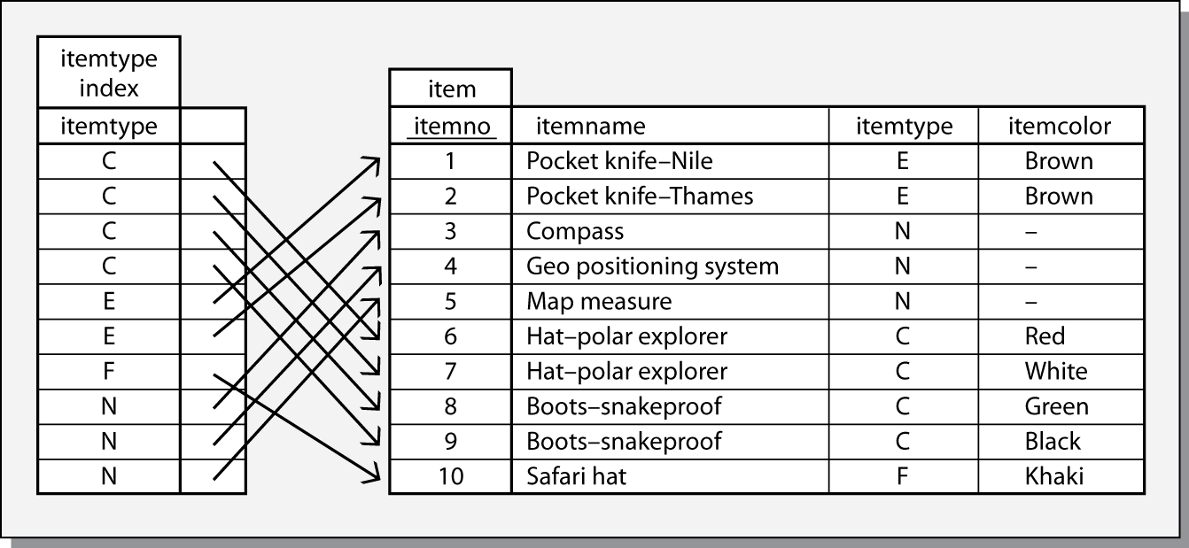
Index
Indexes are used to accelerate data access and ensure uniqueness. An
index is an ordered set of pointers to rows of a base table. Think
of an index as a table that contains two columns. The first column
contains values for the index key, and the second contains a list of
addresses of rows in the table. Since the values in the first column are
ordered (i.e., in ascending or descending sequence), the index table can
be searched quickly. Once the required key has been found in the table,
the row’s address in the second column can be used to retrieve the data
quickly. An index can be specified as being unique, in which case the
RDBMS ensures that the corresponding table does not have rows with
identical index keys.
An example of an index
Notation
A short primer on notation is required before we examine SQL commands.
Text in uppercase is required as is.
Text in lowercase denotes values to be selected by the query writer.
Statements enclosed within square brackets are optional.
| indicates a choice.
An ellipsis ... indicates that the immediate syntactic unit may be
repeated optionally more than once.
Creating a table
CREATE TABLE is used to define a new base table, either interactively or
by embedding the statement in a host language. The statement specifies a
table’s name, provides details of its columns, and provides integrity
checks. The syntax of the command is
CREATE TABLE base-table
    column-definition-block
    [primary-key-block]
    [referential-constraint-block]
    [unique-block];
Column definition
The column definition block defines the columns in a table. Each column
definition consists of a column name, data type, and optionally the
specification that the column cannot contain null values. The general
form is
(column-definition [, ...])
where column-definition is of the form
column-name data-type [NOT NULL]
The NOT NULL clause specifies that the particular column must have a
value whenever a new row is inserted.
Constraints
A constraint is a rule defined as part of CREATE TABLE that defines
valid sets of values for a base table by placing limits on INSERT,
UPDATE, and DELETE operations. Constraints can be named (e.g.,
fk_stock_nation) so that they can be turned on or off and modified.
The four constraint variations apply to primary key, foreign key, unique
values, and range checks.
Primary key constraint
The primary key constraint block specifies a set of columns that
constitute the primary key. Once a primary key is defined, the system
enforces its uniqueness by checking that the primary key of any new row
does not already exist in the table. A table can have only one primary
key. While it is not mandatory to define a primary key, it is good
practice always to define a table’s primary key, though it is not that
common to name the constraint. The general form of the constraint is
[primary-key-name] PRIMARY KEY(column-name [asc|desc] [, ...])
The optional ASC or DESC clause specifies whether the values from this
key are arranged in ascending or descending order, respectively.
For example:
pk_stock PRIMARY KEY(stkcode)
Foreign key constraint
The referential constraint block defines a foreign key, which consists
of one or more columns in the table that together must match a primary
key of the specified table (or else be null). A foreign key value is
null when any one of the columns in the row constituting the foreign key
is null. Once the foreign key constraint is defined, the RDBMS will check
every insert and update to ensure that the constraint is observed. The
general form is
CONSTRAINT constraint-name FOREIGN KEY(column-name [,…])
    REFERENCES table-name(column-name [,…])
        [ON DELETE (RESTRICT | CASCADE | SET NULL)]
The constraint-name defines a referential constraint. You cannot use the
same constraint-name more than once in the same table. Column-name
identifies the column or columns that comprise the foreign key. The data
type and length of foreign key columns must match exactly the data type
and length of the primary key columns. The clause REFERENCES table-name
specifies the name of an existing table, and its primary key, that
contains the primary key, which cannot be the name of the table being
created.
The ON DELETE clause defines the action taken when a row is deleted from
the table containing the primary key. There are three options:
RESTRICT prevents deletion of the primary key row until all
corresponding rows in the related table, the one containing the
foreign key, have been deleted. RESTRICT is the default and the
cautious approach for preserving data integrity.
CASCADE causes all the corresponding rows in the related table also
to be deleted.
SET NULLS sets the foreign key to null for all corresponding rows in
the related table.
For example:
CONSTRAINT fk_stock_nation FOREIGN KEY(natcode)
    REFERENCES nation(natcode)
Unique constraint
A unique constraint creates a unique index for the specified column or
columns. A unique key is constrained so that no two of its values are
equal. Columns appearing in a unique constraint must be defined as NOT
NULL. Also, these columns should not be the same as those of the table’s
primary key, which is guaranteed uniqueness by its primary key
definition. The constraint is enforced by the RDBMS during execution of
INSERT and UPDATE statements. The general format is
UNIQUE constraint-name (column-name [ASC|DESC] [, …])
An example follows:
CONSTRAINT unq_stock_stkname UNIQUE(stkname)
Check constraint
A check constraint defines a set of valid values and can be set for a table or column.
Table constraints are defined in CREATE TABLE and ALTER TABLE
statements. They can be set for one or more columns in a table. A table constraint, for example, might ensure that the selling prices is greater than the cost.
CREATE TABLE item (
  costPrice DECIMAL(9,2),
    sellPrice DECIMAL(9,2),
    CONSTRAINT profit_check CHECK (sellPrice > costPrice));
A column constraint is defined in a CREATE TABLE statement for a single column. In the following case, category is restricted to three values.
CREATE TABLE item (
  category CHAR(1) CONSTRAINT category_constraint
    CHECK (category IN ('B', 'L', 'S')));
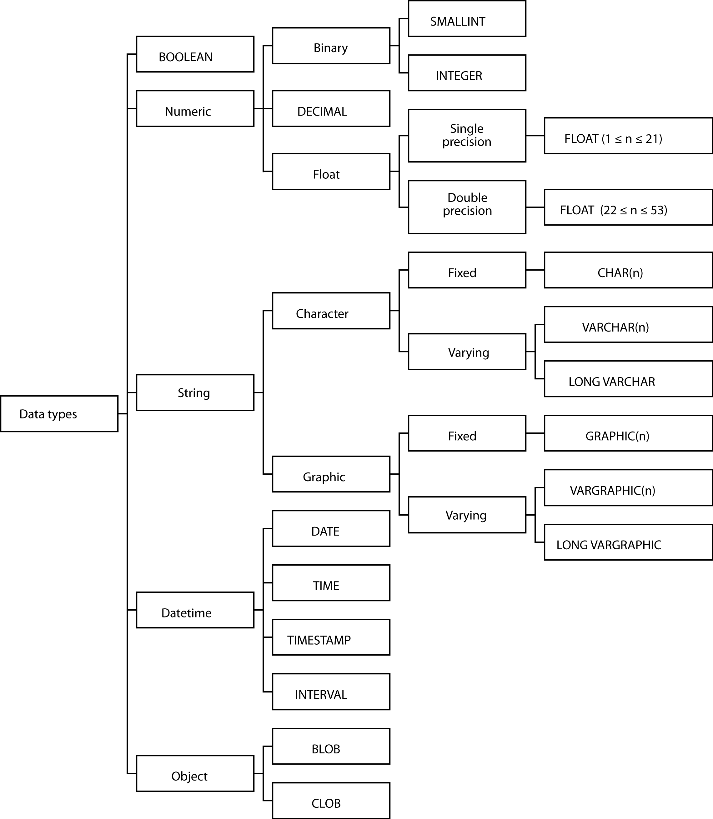
Data types
Some of the variety of data types that can be used are depicted in the
following figure and described in more detail in the following pages.
Data types
BOOLEAN
Boolean data types can have the values true, false, or unknown.
SMALLINT and INTEGER
Most commercial computers have a 32-bit word, where a word is a unit of
storage. An integer can be stored in a full word or half a word. If it
is stored in a full word (INTEGER), then it can be 31 binary digits in
length. If half-word storage is used (SMALLINT), then it can be 15
binary digits long. In each case, one bit is used for the sign of the
number. A column defined as INTEGER can store a number in the range
-231 to 231-1 or -2,147,483,648 to 2,147,483,647. A column defined as SMALLINT can store a number in the range -215 to 215-1 or -32,768 to 32,767. Just remember that INTEGER is good for ±2 billion
and SMALLINT for ±32,000.
FLOAT
Scientists often deal with numbers that are very large (e.g., Avogadro’s
number is 6.02252×10²³) or very small (e.g., Planck’s constant is
6.6262×10⁻³⁴ joule sec). The FLOAT data type is used for storing
such numbers, often referred to as floating-point numbers. A
single-precision floating-point number requires 32 bits and can
represent numbers in the range -7.2×1075 to -5.4×10-79, 0,
5.4×10-79 to 7.2×1075 with a precision of about 7 decimal
digits. A double-precision floating-point number requires 64 bits. The
range is the same as for a single-precision floating-point number. The
extra 32 bits are used to increase precision to about 15 decimal digits.
In the specification FLOAT(n), if n is between 1 and 21 inclusive,
single-precision floating-point is selected. If n is between 22 and 53
inclusive, the storage format is double-precision floating-point. If n
is not specified, double-precision floating-point is assumed.
DECIMAL
Binary is the most convenient form of storing data from a computer’s
perspective. People, however, work with a decimal number system. The
DECIMAL data type is convenient for business applications because data
storage requirements are defined in terms of the maximum number of
places to the left and right of the decimal point. To store the current
value of an ounce of gold, you would possibly use DECIMAL(6,2) because
this would permit a maximum value of $9,999.99. Notice that the general
form is DECIMAL(p,q), where p is the total number of digits in the
column, and q is the number of digits to the right of the decimal point.
CHAR and VARCHAR
Nonnumeric columns are stored as character strings. A person’s family
name is an example of a column that is stored as a character string.
CHAR(n) defines a column that has a fixed length of n characters, where
n can be a maximum of 255.
When a column’s length can vary greatly, it makes sense to define the
field as VARCHAR. A column defined as VARCHAR consists of two parts: a
header indicating the length of the character string and the string. If
a table contains a column that occasionally stores a long string of text
(e.g., a message field), then defining it as VARCHAR makes sense.
VARCHAR can store strings up to 65,535 characters long.
Why not store all character columns as VARCHAR and save space? There is
a price for using VARCHAR with some relational systems. First,
additional space is required for the header to indicate the length of
the string. Second, additional processing time is required to handle a
variable-length string compared to a fixed-length string. Depending on
the RDBMS and processor speed, these might be important considerations,
and some systems will automatically make an appropriate choice. For
example, if you use both data types in the same table, MySQL will
automatically change CHAR into VARCHAR for compatibility reasons.
There are some columns where there is no trade-off because all
possible entries are always the same length. Canadian postal codes, for
instance, are always six characters (e.g., the postal code for Ottawa is
K1A0A1).
Data compression is another approach to the space wars problem. A
database can be defined with generous allowances for fixed-length
character columns so that few values are truncated. Data compression can
be used to compress the file to remove wasted space. Data compression,
however, is slow and will increase the time to process queries. You save
space at the cost of time, and save time at the cost of space. When
dealing with character fields, the database designer has to decide
whether time or space is more important.
Times and dates
Columns that have a data type of DATE are stored as yyyymmdd (e.g.,
2022-11-04 for November 4, 2022). There are two reasons for this format.
First, it is convenient for sorting in chronological order. The common
American way of writing dates (mmddyy) requires processing before
chronological sorting. Second, the full form of the year should be
recorded for exactness.
For similar reasons, it makes sense to store times in the form hhmmss
with the understanding that this is 24-hour time (also known as European
time and military time). This is the format used for data type TIME.
Some applications require precise recording of events. For example,
transaction processing systems typically record the time a transaction
was processed by the system. Because computers operate at high speed,
the TIMESTAMP data type records date and time with microsecond accuracy.
A timestamp has seven parts: year, month, day, hour, minute, second,
and microsecond. Date and time are defined as previously described
(i.e., yyyymmdd and hhmmss, respectively). The range of the
microsecond part is 000000 to 999999.
Although times and dates are stored in a particular format, the
formatting facilities that generally come with a RDBMS usually allow
tailoring of time and date output to suit local standards. Thus for a
U.S. firm, date might appear on a report in the form mm/dd/yy; for a
European firm following the ISO standard, date would appear as
yyyy-mm-dd.
SQL-99 introduced the INTERVAL data type, which is a single value
expressed in some unit or units of time (e.g., 6 years, 5 days, 7
hours).
BLOB (binary large object)
BLOB is a large-object data type that stores any kind of binary data.
Binary data typically consists of a saved spreadsheet, graph, audio
file, satellite image, voice pattern, or any digitized data. The BLOB
data type has no maximum size.
CLOB (character large object)
CLOB is a large-object data type that stores any kind of character data.
Text data typically consists of reports, correspondence, chapters of a
manual, or contracts. The CLOB data type has no maximum size.
❓ Skill builder
What data types would you recommend for the following?
A book’s ISBN
A photo of a product
The speed of light (2.9979 × 10⁸ meters per second)
A short description of an animal’s habitat
The title of a Japanese book
A legal contract
The status of an electrical switch
The date and time a reservation was made
An item’s value in euros
The number of children in a family
Collation sequence
A RDBMS will typically support many character sets. so it can handle text
in different languages. While many European languages are based on an
alphabet, they do not all use the same alphabet. For example, Norwegian
has some additional characters (e.g., æ ,ø, å) compared to English, and
French accents some letters (e.g., é, ü, and ȃ), which do not occur in
English. Alphabet based languages have a collating sequence, which
defines how to sort individual characters in a particular language. For
English, it is the familiar A B C … X Y Z. Norwegian’s collating
sequence includes three additional symbols, and the sequence is A B C
… X Y Z Æ Ø Å. When you define a database you need to define its
collating sequence. Thus, a database being set up for exclusive use in
Chile would opt for a Spanish collating sequence. You can specify a
collation sequence at the database, table, and, column level. The usual
practice is to specify at the database level.
CREATE DATABASE ClassicModels COLLATE latin1_general_cs;
The latin1_general character set is suitable for Western European
languages. The cs suffix indicates that comparisons are case
sensitive. In other words, a query will see the two strings ‘abc’ and
‘Abc’ as different, whereas if case sensitivity is turned off, the
strings are considered identical. Case sensitivity is usually the right
choice to ensure precision of querying.
Scalar functions
Most implementations of SQL include functions that can be used in
arithmetic expressions, and for data conversion or data extraction. The
following sampling of these functions will give you an idea of what is
available. You will need to consult the documentation for your version
of SQL to determine the functions it supports. For example, Microsoft
SQL Server has more than 100 additional functions.
Some examples of SQL’s built-in scalar functions
| CURRENT_DATE() |
Retrieves the current date |
| EXTRACT(date_time_part FROM expression) |
Retrieves part of a time or date (e.g., YEAR, MONTH, DAY, HOUR, MINUTE, or SECOND) |
| SUBSTRING(str, pos, len) |
Retrieves a string of length len starting at position pos from string str |
Some examples for you to run
SELECT extract(day) FROM CURRENT_DATE());
SELECT SUBSTRING(`person first`, 1,1), `person last` FROM person;
A vendor’s additional functions can be very useful. Remember, though,
that use of a vendor’s extensions might limit portability.
How many days’ sales are stored in the sale table?
This sounds like a simple query, but you have to do a self-join and also
know that there is a function, DATEDIFF, to determine the number of days
between any two dates. Consult your RDBMS manual to learn about other
functions for dealing with dates and times.
WITH
late AS (SELECT * FROM sale),
early AS (SELECT * FROM sale)
SELECT DISTINCT DATEDIFF(late.saledate,early.saledate) AS Difference
    FROM late JOIN early
        ON late.saledate =
            (SELECT MAX(saledate) FROM sale)
        AND early.saledate =
            (SELECT MIN(saledate) FROM sale);
The preceding query is based on the idea of joining sale with a copy
of itself. The matching column from late is the latest sale’s date (or
MAX), and the matching column from early is the earliest sale’s date
(or MIN). As a result of the join, each row of the new table has both
the earliest and latest dates.
Table commands
Altering a table
The ALTER TABLE statement has two purposes. First, it can add a single
column to an existing table. Second, it can add, drop, activate, or
deactivate primary and foreign key constraints. A base table can be
altered by adding one new column, which appears to the right of existing
columns. The format of the command is
ALTER TABLE base-table ADD column data-type;
Notice that there is no optional NOT NULL clause for column-definition
with ALTER TABLE. It is not allowed because the ALTER TABLE statement
automatically fills the additional column with null in every case. If
you want to add multiple columns, you repeat the command. ALTER TABLE
does not permit changing the width of a column or amending a column’s
data type. It can be used for deleting an unwanted column.
ALTER TABLE stock ADD stkrating CHAR(3);
ALTER TABLE is also used to change the status of referential
constraints. You can deactivate constraints on a table’s primary key or
any of its foreign keys. Deactivation also makes the relevant tables
unavailable to everyone except the table’s owner or someone possessing
database management authority. After the data are loaded, referential
constraints must be reactivated before they can be automatically
enforced again. Activating the constraints enables the RDBMS to validate
the references in the data.
Dropping a table
A base table can be deleted at any time by using the DROP statement. The
format is
The table is deleted, and any views or indexes defined on the table are
also deleted.
Creating a view
A view is a virtual table. It has no physical counterpart but appears to
the client as if it really exists. A view is defined in terms of other
tables that exist in the database. The syntax is
CREATE VIEW view [column [,column] …)]
    AS subquery;
There are several reasons for creating a view. First, a view can
be used to restrict access to certain rows or columns. This is
particularly important for sensitive data. An organization’s person
table can contain both private data (e.g., annual salary) and public
data (e.g., office phone number). A view consisting of public data
(e.g., person’s name, department, and office telephone number) might be
provided to many people. Access to all columns in the table, however,
might be confined to a small number of people. Here is a sample view
that restricts access to a table.
CREATE VIEW stklist
    AS SELECT stkfirm, stkprice FROM stock;
Handling derived data is a second reason for creating a view. A column
that can be computed from one or more other columns should always be
defined by a view. Thus, a stock’s yield would be computed by a view
rather than defined as a column in a base table.
CREATE VIEW stk
    (stkfirm, stkprice, stkqty, stkyield)
    AS SELECT stkfirm, stkprice, stkqty, stkdiv/stkprice*100
        FROM stock;
A third reason for defining a view is to avoid writing common SQL
queries. For example, there may be some joins that are frequently part
of an SQL query. Productivity can be increased by defining these joins
as views. Here is an example:
CREATE VIEW stkvalue
    (nation, firm, price, qty, value)
    AS SELECT natname, stkfirm, stkprice*exchrate, stkqty,
        stkprice*exchrate*stkqty FROM stock JOIN nation
            ON stock.natcode = nation.natcode;
The preceding example demonstrates how CREATE VIEW can be used to rename
columns, create new columns, and involve more than one table. The column
nation corresponds to natname, firm to stkfirm, and so forth. A
new column, price, is created that converts all share prices from the
local currency to British pounds.
Data conversion is a fourth useful reason for a view. The United
States is one of the few countries that does not use the metric system,
and reports for American managers often display weights and measures in
pounds and feet, respectively. The database of an international company
could record all measurements in metric format (e.g., weight in
kilograms) and use a view to convert these measures for American
reports.
When a CREATE VIEW statement is executed, the definition of the view is
entered in the systems catalog. The subquery following AS, the view
definition, is executed only when the view is referenced in an SQL
command. For example, the following command would enable the subquery to
be executed and the view created:
SELECT * FROM stkvalue WHERE price > 10;
SELECT natname, stkfirm, stkprice*exchrate, stkqty, stkprice*exchrate*stkqty
    FROM stock JOIN nation
        ON stock.natcode = nation.natcode
        WHERE stkprice*exchrate > 10;
Any table that can be defined with a SELECT statement is a potential
view. Thus, it is possible to have a view that is defined by another
view.
Dropping a view
DROP VIEW is used to delete a view from the system catalog. A view might
be dropped because it needs to be redefined or is no longer used. It
must be dropped before a revised version of the view is created.
The syntax is
Remember, if a base table is dropped, all views based on that table are
also dropped.
Creating an index
An index helps speed up retrieval (a more detailed discussion of
indexing is covered later in this book). A column that is frequently
referred to in a WHERE clause is a possible candidate for indexing. For
example, if data on stocks were frequently retrieved using stkfirm,
then this column should be considered for an index. The format for
CREATE INDEX is
CREATE [UNIQUE] INDEX indexname
    ON base-table (column [order] [,column, [order]] …)
    [CLUSTER];
This next example illustrates use of CREATE INDEX.
CREATE UNIQUE INDEX stkfirmindx ON stock(stkfirm);
In the preceding example, an index called stkfirmindx is created for
the table stock. Index entries are ordered by ascending (the default
order) values of stkfirm. The optional clause UNIQUE specifies that no
two rows in the base table can have the same value for stkfirm, the
indexed column. Specifying UNIQUE means that the RDBMS will reject any
insert or update operation that would create a duplicate value for
stkfirm.
A composite index can be created from several columns, which is often
necessary for an associative entity. The following example illustrates
the creation of a composite index.
CREATE INDEX lineitemindx ON lineitem (lineno, saleno);
Dropping an index
Indexes can be dropped at any time by using the DROP INDEX statement.
The general form of this statement is
Data manipulation
SQL supports four DML statements—SELECT, INSERT, UPDATE, and DELETE.
Each of these is discussed in turn, with most attention focusing on
SELECT because of the variety of ways in which it can be used. First, we
need to understand why we must qualify column names and temporary names.
Qualifying column names
Ambiguous references to column names are avoided by qualifying a column
name with its table name, especially when the same column name is used
in several tables. Clarity is maintained by prefixing the column name
with the table name. The following example demonstrates qualification of
the natcode, which appears in both stock and nation.
SELECT stkfirm, stkprice FROM stock JOIN nation
    ON stock.natcode = nation.natcode;
Temporary names
Using the WITH clause, a table or view can be given a temporary name, or
alias, that remains current for a query. Temporary names are used in a
self-join to distinguish the copies of the table.
WITH
wrk AS (SELECT * FROM emp),
boss AS (SELECT * FROM emp)
SELECT wrk.empfname
    FROM wrk JOIN boss
        ON wrk.bossno = boss.empno;
A temporary name also can be used as a shortened form of a long table
name. For example, l might be used merely to avoid having to enter
lineitem more than once. If a temporary name is specified for a table
or view, any qualified reference to a column of the table or view must
also use that temporary name.
SELECT
The SELECT statement is by far the most interesting and challenging of
the four DML statements. It reveals a major benefit of the relational
model: powerful interrogation capabilities. It is challenging because
mastering the power of SELECT requires considerable practice with a wide
range of queries. The major varieties of SELECT are presented in this
section. The SQL Playbook, on the book’s website, reveals the full
power of the command.
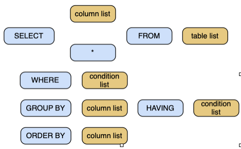
The general format of SELECT is
SELECT [DISTINCT] item(s) FROM table(s)
    [WHERE condition]
    [GROUP BY column(s)] [HAVING condition]
    [ORDER BY column(s)];
Alternatively, we can diagram the structure of SELECT.
Structure of SELECT
Product
Product, or more strictly Cartesian product, is a fundamental operation
of relational algebra. It is rarely used by itself in a query; however,
understanding its effect helps in comprehending join. The product of two
tables is a new table consisting of all rows of the first table
concatenated with all possible rows of the second table. For example:
Form the product of stock and nation.
SELECT * FROM stock, nation;
Run the query and observe that the new table contains 64 rows (16*4), where stock has 16 rows and nation has 4 rows. It has 10 columns (7 + 3), where stock has 7 columns and nation has 3 columns. Note that each row in stock is concatenated
with each row in nation.
Find the percentage of Australian stocks in the portfolio.
To answer this query, you need to count the number of Australian stocks,
count the total number of stocks in the portfolio, and then compute the
percentage. Computing each of the totals is a straightforward
application of COUNT. If we save the results of the two counts as views,
then we have the necessary data to compute the percentage. The two views
each consist of a single-cell table (i.e., one row and one column). We
create the product of these two views to get the data needed for
computing the percentage in one row. The SQL is
CREATE VIEW austotal (auscount) AS
  SELECT COUNT(*) FROM nation JOIN stock
     ON natname = 'Australia'
     WHERE nation.natcode = stock.natcode;
CREATE VIEW total (totalcount) AS
  SELECT COUNT(*) FROM stock;
SELECT auscount/totalcount*100
  AS percentage FROM austotal, total;
CREATE VIEW total (totalcount) AS
    SELECT COUNT(*) FROM stock;
SELECT auscount*100/totalcount as Percentage
    FROM austotal, total;
The result of a COUNT is always an integer, and SQL will typically
create an integer data type in which to store the results. When two
variables have a data type of integer, SQL will likely use integer
arithmetic for all computations, and all results will be integer. To get
around the issue of integer arithmetic, we first multiply the number of
Australian stocks by 100 before dividing by the total number of stocks.
Because of integer arithmetic, you might get a different answer if you
use the following SQL.
SELECT auscount/totalcount*100 as Percentage
    FROM austotal, total;
The preceding example was used to show when you might find product
useful. You can also write the query as
SELECT (SELECT COUNT(*) FROM stock WHERE natcode = 'AUS')*100/
    (SELECT COUNT(*) FROM stock) as Percentage;
Inner join
Inner join, often referred to as join, is a powerful and frequently used
operation. It creates a new table from two existing tables by matching
on a column common to both tables. An equijoin is the simplest form
of join; in this case, columns are matched on equality.
SELECT * FROM stock JOIN nation
    ON stock.natcode = nation.natcode;
There are other ways of expressing join that are more concise. For
example, we can write
SELECT * FROM stock INNER JOIN nation USING (natcode);
The preceding syntax implicitly recognizes the frequent use of the same
column name for matching primary and foreign keys.
A further simplification is to rely on the primary and foreign key
definitions to determine the join condition, so we can write
SELECT * FROM stock NATURAL JOIN nation;
An equijoin creates a new table that contains two identical columns. If
one of these is dropped, then the remaining table is called a natural
join.
Theta join
As you now realize, join can be thought of as a product with a condition
clause. There is no reason why this condition needs to be restricted to
equality. There could easily be another comparison operator between the
two columns. This general version is called a theta-join because theta
is a variable that can take any value from the set ‘=’, ‘<’, ‘<=’,
‘>’, and ‘>=’.
As you discovered earlier, there are occasions when you need to join a
table to itself. To do this, make two copies of the table and give
each of them a unique name.
Find the names of employees who earn more than their boss.
WITH wrk AS (SELECT * FROM emp),
     boss AS (SELECT * FROM emp)
SELECT wrk.empfname AS Worker, wrk.empsalary AS Salary,
  boss.empfname AS Boss, boss.empsalary AS Salary
FROM wrk JOIN boss
    ON wrk.bossno = boss.empno
    WHERE wrk.empsalary > boss.empsalary;
Table 10.1: 1 records
| Sarah |
56000 |
Brier |
43000 |
Outer join
An inner join reports those rows where the primary and foreign keys match. There are also situations where you might want an outer join, which comes in three flavors as shown in the following figure.
Types of joins
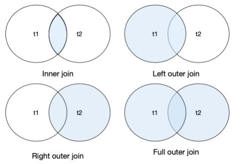
A traditional join, more formally known as an inner join, reports those rows where the primary and foreign keys match. An outer join reports these matching rows and other rows depending on which form is used, as the following examples illustrate for the sample table.
| id |
col1 |
|
id |
col2 |
| 1 |
a |
|
1 |
x |
| 2 |
b |
|
3 |
y |
| 3 |
c |
|
5 |
z |
A left outer join is an inner join plus those rows from t1 not
included in the inner join.
SELECT id, col1, col2 FROM t1 LEFT JOIN t2 USING (id)
Here is an example to illustrate the use of a left join.
For all brown items, report each sale. Include in the report those
brown items that have appeared in no sales.
SELECT itemname, saleno, lineqty FROM item
    LEFT JOIN lineitem USING (itemno)
        WHERE itemcolor = 'Brown'
        ORDER BY itemname;
A right outer join is an inner join plus those rows from t2 not
included in the inner join.
SELECT id, col1, col2 FROM t1 RIGHT JOIN t2 USING (id);
A full outer join is an inner join plus those rows from t1 and t2
not included in the inner join.
SELECT id, col1, col2 FROM t1 FULL JOIN t2 USING (id);
| 1 |
a |
x |
| 2 |
b |
null |
| 3 |
c |
y |
| 5 |
null |
z |
MySQL does not support a full outer join, rather you must use a union of
left and right outer joins.
SELECT id, col1, col2 FROM t1 LEFT JOIN t2 USING (id)
UNION
SELECT id, col1, col2 FROM t1 RIGHT JOIN t2 USING (id);
Simple subquery
A subquery is a query within a query. There is a SELECT statement nested
inside another SELECT statement. Simple subqueries were used extensively
in earlier chapters. For reference, here is a simple subquery used
earlier:
SELECT stkfirm FROM stock
    WHERE natcode IN
        (SELECT natcode FROM nation
            WHERE natname = 'Australia');
Aggregate functions
SQL’s aggregate functions increase its retrieval power. These functions
were covered earlier and are only mentioned briefly here for
completeness. The five aggregate functions are shown in the following
table. Nulls in the column are ignored in the case of SUM, AVG, MAX, and
MIN. COUNT(*) does not distinguish between null and non-null values in
a column. Use COUNT(columnname) to exclude a null value in columnname.
Aggregate functions
| COUNT |
Counts the number of values in a column |
| SUM |
Sums the values in a column |
| AVG |
Determines the average of the values in a column |
| MAX |
Determines the largest value in a column |
| MIN |
Determines the smallest value in a column |
GROUP BY and HAVING
The GROUP BY clause is an elementary form of control break reporting and
supports grouping of rows that have the same value for a specified
column and produces one row for each different value of the grouping
column. For example,
Report by nation the total value of stockholdings.
SELECT natname, SUM(stkprice*stkqty*exchrate) AS total
    FROM stock JOIN nation ON stock.natcode = nation.natcode
        GROUP BY natname;
The HAVING clause is often associated with GROUP BY. It can be thought
of as the WHERE clause of GROUP BY because it is used to eliminate rows
for a GROUP BY condition. Both GROUP BY and HAVING are dealt with
in-depth in Chapter 4.
REGEXP
The REGEXP clause supports pattern matching to find a defined set of
strings in a character column (CHAR or VARCHAR). Refer to Chapters 3 and
4 for more details.
CASE
The CASE statement is used to implement a series of conditional clauses. In the following query, the first step creates a temporary table that records customers and their total orders. The second step classifies customers into four categories based on their total orders.
WITH temp AS
  (SELECT customerName, COUNT(*) AS orderCount
    FROM Orders JOIN Customers
      ON Customers.customerNumber = Orders.customerNumber
      GROUP BY customerName)
SELECT customerName, orderCount,
    CASE orderCount
      WHEN 1 THEN 'One-time Customer'
      WHEN 2 THEN 'Repeated Customer'
      WHEN 3 THEN 'Frequent Customer'
      ELSE 'Loyal Customer'
    end customerType
    FROM temp
ORDER BY customerName;
INSERT
There are two formats for INSERT. The first format is used to insert one
row into a table.
Inserting a single record
The general form is
INSERT INTO table [(column [,column] …)]
    VALUES (literal [,literal] …);
For example,
INSERT INTO stock
    (stkcode,stkfirm,stkprice,stkqty,stkdiv,stkpe)
    VALUES ('FC','Freedonia Copper',27.5,10529,1.84,16);
In this example, stkcode is given the value “FC,” stkfirm is
“Freedonia Copper,” and so on. The nth column in the table
is the nth value in the list.
When the value list refers to all field names in the left-to-right order
in which they appear in the table, then the columns list can be omitted.
So, it is possible to write the following:
INSERT INTO stock
    VALUES ('FC','Freedonia Copper',27.5,10529,1.84,16);
If some values are unknown, then the INSERT can omit these from the
list. Undefined columns will have nulls. For example, if a new stock is
to be added for which the PE ratio is 5, the
following INSERT statement would be used:
INSERT INTO stock
    (stkcode, stkfirm, stkPE)
    VALUES ('EE','Elysian Emeralds',5);
Inserting multiple records using a query
The second form of INSERT operates in conjunction with a subquery. The
resulting rows are then inserted into a table. Imagine the situation
where stock price information is downloaded from an information service
into a table. This table could contain information about all stocks and
may contain additional columns that are not required for the stock
table. The following INSERT statement could be used:
INSERT INTO stock
    (stkcode, stkfirm, stkprice, stkdiv, stkpe)
    SELECT code, firm, price, div, pe
    FROM download WHERE code IN
    ('FC','PT','AR','SLG','ILZ','BE','BS','NG','CS','ROF');
Think of INSERT with a subquery as a way of copying a table. You can
select the rows and columns of a particular table that you want to copy
into an existing or new table.
UPDATE
The UPDATE command is used to modify values in a table. The general
format is
UPDATE table
    SET column = scalar expression
        [, column = scalar expression] …
    [WHERE condition];
Permissible scalar expressions involve columns, scalar functions (see
the section on scalar functions in this chapter), or constants. No
aggregate functions are allowable.
Updating a single row
UPDATE can be used to modify a single row in a table. Suppose you need
to revise your data after 200,000 shares of Minnesota Gold are sold. You
would code the following:
UPDATE stock
    SET stkqty = stkqty - 200000
    WHERE stkcode = 'MG';
Updating multiple rows
Multiple rows in a table can be updated as well. Imagine the situation
where several stocks change their dividend to £2.50. Then the following
statement could be used:
UPDATE stock
    SET stkdiv = 2.50
    WHERE stkcode IN ('FC','BS','NG');
Updating all rows
All rows in a table can be updated by simply omitting the WHERE clause.
To give everyone a 5 percent raise, use
UPDATE emp
    SET empsalary = empsalary*1.05;
Updating with a subquery
A subquery can also be used to specify which rows should be changed.
Consider the following example. The employees in the departments on the
fourth floor have won a productivity improvement
bonus of 10 percent. The following SQL statement would update their
salaries:
UPDATE emp
    SET empsalary = empsalary*1.10
    WHERE deptname IN
        (SELECT deptname FROM dept WHERE deptfloor = 4);
DELETE
The DELETE statement erases one or more rows in a table. The general
format is
DELETE FROM table
    [WHERE condition];
Delete a single record
If all stocks with stkcode equal to “BE” were sold, then this row can be
deleted using
DELETE FROM stock WHERE stkcode = 'BE';
Delete multiple records
If all Australian stocks were liquidated, then the following command
would delete all the relevant rows:
DELETE FROM stock
    WHERE natcode in
    (SELECT natcode FROM nation WHERE natname = 'Australia');
Delete all records
All records in a table can be deleted by omitting the WHERE clause. The
following statement would delete all rows if the entire portfolio were
sold:
This command is not the same as DROP TABLE because, although the table
is empty, it still exists.
Delete with a subquery
Despite their sterling efforts in the recent productivity drive, all the
employees on the fourth floor have been fired (the
rumor is that they were fiddling the tea money). Their records can be
deleted using
DELETE FROM emp
    WHERE deptname IN
        (SELECT deptname FROM dept WHERE deptfloor = 4);
SQL routines
SQL provides two types of routines—functions and procedures—that are
created, altered, and dropped using standard SQL. Routines add
flexibility, improve programmer productivity, and facilitate the
enforcement of business rules and standard operating procedures across
applications.
SQL function
A function is SQL code that returns a value when invoked within an SQL
statement. It is used in a similar fashion to SQL’s built-in functions.
Consider the case of an Austrian firm with a database in which all
measurements are in SI units (e.g., meters). Because its U.S. staff is
not familiar with SI, it decides to implement a series of
user-defined functions to handle the conversion. Here is the function
for converting from kilometers to miles. Note that MySQL requires that you include the word DETERMINISTIC for a function that always produces the same result for the same input parameters.
CREATE FUNCTION km_to_miles(km REAL)
    RETURNS REAL
    DETERMINISTIC
    RETURN 0.6213712*km;
The preceding function can be used within any SQL statement to make the
conversion. For example:
❓ Skill builder
Create a table containing the average daily temperature in Tromsø,
Norway, then write a function to convert Celsius to Fahrenheit (F =
C*1.8 + 32), and test the function by reporting temperatures in C and
F.
The temperatures in month order:
-4.7, -4.1, -1.9, 1.1, 5.6, 10.1, 12.7, 11.8, 7.7, 2.9, -1.5, -3.7
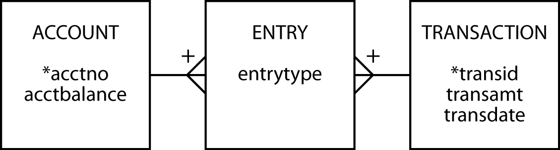
SQL procedure
A procedure is SQL code that is dynamically loaded and executed by a
CALL statement, usually within a database application. We use an
accounting system to demonstrate the features of a stored procedure, in
which a single accounting transaction results in two entries (one debit
and one credit). In other words, a transaction has multiple entries, but
an entry is related to only one transaction. An account (e.g., your bank
account) has multiple entries, but an entry is for only one account.
Considering this situation results in the following data model.
A simple accounting system
The following are a set of steps for processing a transaction (e.g.,
transferring money from a checking account to a money market account):
Write the transaction to the transaction table so you have a record
of the transaction.
Update the account to be credited by incrementing its balance in the
account table.
Insert a row in the entry table to record the credit.
Update the account to be debited by decrementing its balance in the
account table.
Insert a row in the entry table to record the debit.
Here is the code for a stored procedure to execute these steps. Note
that the first line sets the delimiter to // because the default
delimiter for SQL is a semicolon (;), which we need to use to delimit
the multiple SQL commands in the procedure. The last statement in the
procedure is thus END // to indicate the end of the procedure.
DELIMITER //
-- Define the input values
CREATE PROCEDURE transfer (
IN `Credit account` INTEGER,
IN `Debit account`  INTEGER,
IN  Amount          DECIMAL(9,2),
IN `Transaction ID` INTEGER)
LANGUAGE SQL
DETERMINISTIC
BEGIN
-- Save the transaction details
INSERT INTO transaction VALUES (`Transaction ID`, Amount, CURRENT_DATE);
UPDATE account
-- Increase the credit account
SET acctbalance = acctbalance + Amount
WHERE acctno = `Credit account`;
INSERT INTO entry VALUES (`Transaction ID`, `Credit account`, 'cr');
UPDATE account
-- Decrease the debit account
SET acctbalance = acctbalance - Amount
WHERE acctno = `Debit account`;
INSERT INTO entry VALUES (`Transaction ID`, `Debit account`, 'db');
END //
A CALL statement executes a stored procedure. The generic CALL statement
for the preceding procedure is
CALL transfer(cracct, dbacct, amt, transno);
Thus, imagine that transaction 1005 transfers $100 to account 1 (the
credit account) from account 2 (the debit account). The specific call is
CALL transfer(1,2,100,1005);
❓ Skill builder
Create the tables for the preceding data model, insert a some reows,
and enter the code for the stored procedure. Now, test the stored
procedure and query the tables to verify that the procedure has
worked.
Write a stored procedure to add details of a gift to the donation
database (see exercises in Chapter 5).
Trigger
A trigger is a form of stored procedure that executes automatically when
a table’s rows are modified. Triggers can be defined to execute either
before or after rows are inserted into a table, when rows are deleted
from a table, and when columns are updated in the rows of a table.
Triggers can include virtual tables that reflect the row image before
and after the operation, as appropriate. Triggers can be used to enforce
business rules or requirements, integrity checking, and automatic
transaction logging.
Consider the case of recording all updates to the stock table (see
Chapter 4). First, you must define a table in which to record details of
the change.
CREATE TABLE stock_log (
stkcode           CHAR(3),
old_stkprice      DECIMAL(6,2),
new_stkprice      DECIMAL(6,2),
old_stkqty        DECIMAL(8),
new_stkqty        DECIMAL(8),
update_stktime  TIMESTAMP NOT NULL,
    PRIMARY KEY(update_stktime));
The trigger writes a record to stock_log every time an update is made
to stock. Two virtual tables (old and new) have details of the prior and current values of stock price (old.stkprice and
new.stkprice) and stock quantity (old.stkprice and new.stkprice).
The INSERT statement also writes the stock’s identifying code and the
time of the transaction.
DELIMITER //
CREATE TRIGGER stock_update
AFTER UPDATE ON stock
FOR EACH ROW BEGIN
INSERT INTO stock_log VALUES
    (OLD.stkcode, OLD.stkprice, NEW.stkprice, OLD.stkqty, NEW.stkqty, CURRENT_TIMESTAMP);
END //
❓ Skill builder
Why is the primary key of stock_log not the same as
that of stock?
Universal Unique Identifier (UUID)
A Universally Unique Identifier (UUID) is a generated number that is globally unique even if generated by independent programs on different computers. The probability that a UUID is not unique is close enough to zero to be negligible. More precisely, the probability of a duplicate within 103 trillion UUIDs is one in a billion.
A UUID is a 128-bit number generated by combining a timestamp and the generating computers’s node id to create an identifier that it temporally and spatially different. A UUID is useful when you want to support different programs on different computers inserting rows in a distributed database.
SELECT UUID() AS UUID_Value;
Security
Data are a valuable resource for nearly every organization. Just as an
organization takes measures to protect its physical assets, it also
needs to safeguard its electronic assets—its organizational memory,
including databases. Furthermore, it often wants to limit the access of
authorized users to particular parts of a database and restrict their
actions to particular operations.
Two SQL features are used to administer security procedures. A view,
discussed earlier in this chapter, can restrict a client’s access to
specified columns or rows in a table, and authorization commands can
establish a user’s privileges.
The authorization subsystem is based on the concept of a privilege—the
authority to perform an operation. For example, a person cannot update a
table unless they have been granted the appropriate update privilege. The
database administrator (DBA) is a master of the universe and has the
highest privilege. The DBA can perform any legal operation. The creator
of an object, say a base table, has full privileges for that object.
Those with privileges can then use GRANT and REVOKE, commands included
in SQL’s data control language (DCL) to extend privileges to or rescind
them from other users.
GRANT
The GRANT command defines a client’s privileges. The general format of
the statement is
GRANT privileges ON object TO users [WITH GRANT OPTION];
where “privileges” can be a list of privileges or the keyword ALL
PRIVILEGES, and “users” is a list of user identifiers or the keyword
PUBLIC. An “object” can be a base table or a view.
The following privileges can be granted for tables and views: SELECT,
UPDATE, DELETE, and INSERT.
The UPDATE privilege specifies the particular columns in a base table or
view that may be updated. Some privileges apply only to base tables.
These are ALTER and INDEX.
The following examples illustrate the use of GRANT:
Give Alice all rights to the stock table.
GRANT ALL PRIVILEGES ON stock TO alice;
Permit the accounting staff, Todd and Nancy, to update the price of a
stock.
GRANT UPDATE (stkprice) ON stock TO todd, nancy;
Give all staff the privilege to select rows from item.
GRANT SELECT ON item TO PUBLIC;
Give Alice all rights to view stk.
GRANT SELECT, UPDATE, DELETE, INSERT ON stk TO alice;
The WITH GRANT OPTION clause
The WITH GRANT OPTION command allows a client to transfer his privileges
to another client, as this next example illustrates:
Give Ned all privileges for the item table and permit him to grant any
of these to other staff members who may need to work with item.
GRANT ALL PRIVILEGES ON item TO ned WITH GRANT OPTION;
This means that Ned can now use the GRANT command to give other staff
privileges. To give Andrew permission for select and insert on item, for
example, Ned would enter
GRANT SELECT, INSERT ON item TO andrew;
REVOKE
What GRANT granteth, REVOKE revoketh. Privileges are removed using the
REVOKE statement. The general format of this statement is
REVOKE privileges ON object FROM users;
These examples illustrate the use of REVOKE.
Remove Sophie’s ability to select from item.
REVOKE SELECT ON item FROM sophie;
Nancy is no longer permitted to update stock prices.
REVOKE UPDATE ON stock FROM nancy;
Cascading revoke
When a REVOKE statement removes a privilege, it can result in more than
one revocation. An earlier example illustrated how Ned used his WITH
GRANT OPTION right to authorize Andrew to select and insert rows on
item. The following REVOKE command
REVOKE INSERT ON item FROM ned;
automatically revokes Andrew’s insert privilege.
The system catalog
The system catalog describes a relational database. It contains the
definitions of base tables, views, indexes, and so on. The catalog
itself is a relational database and can be interrogated using SQL.
Tables in the catalog are called system tables to distinguish them
from base tables, though conceptually these tables are the same. In
MySQL, the system catalog is called information_schema. Some important
system tables in this schema are tables, and columns, and these are used
in the following examples. Note that the names of the system catalog
tables vary with RDBMS implementations, so while the following examples
illustrate use of system catalog tables, it is likely that you will have
to change the table names for other RDBMSs.
The table TABLES contains details of all tables in the database. There
is one row for each table in the database.
Find the table(s) with the most columns.
SELECT table_name, table_rows
    FROM information_schema.tables
        WHERE table_rows = (SELECT MAX(table_rows)
            FROM information_schema.tables);
The COLUMN table stores details about each column in the database.
What columns in what tables store dates?
SELECT table_name, column_name
    FROM information_schema.columns
        WHERE DATA_TYPE = 'date'
            ORDER BY table_name, column_name;
As you can see, querying the catalog is the same as querying a database.
This is a useful feature because you can use SQL queries on the catalog
to find out more about a database.
Natural language processing
Infrequent inquirers of a relational database may be reluctant to use
SQL because they don’t use it often enough to remain familiar with the
language. While the QBE approach can make querying easier, a more
natural approach is to use standard English. In this case, natural
language processing (NLP) is used to convert ordinary English into SQL
so the query can be passed to the relational database. The example in
the table below shows the successful translation of a query to SQL. A
natural language processor must translate a request to SQL and request
clarification where necessary.
An example of natural language processing
| Which movies have won best foreign film sorted by year? |
SELECT DISTINCT [Year], [Title] FROM [Awards] INNER JOIN [Movies] ON [Movies].[Movie ID] = [Awards].[Movie ID] WHERE [Category]=‘Best Foreign Film’ and [Status]=‘Winner’ ORDER BY [Year] ASC; |
Connectivity and ODBC
Over time and because of differing needs, an organization is likely to
purchase RDBMS software from a variety of vendors. Also, in some
situations, mergers and acquisitions can create a multivendor RDBMS
environment. Consequently, the SQL Access Group developed SQL Call-Level
Interface (CLI), a unified standard for remote database access. The
intention of CLI is to provide programmers with a generic approach for
writing software that accesses a database. With the appropriate CLI
database driver, any RDBMS server can provide access to client programs
that use the CLI. On the server side, the RDBMS CLI driver is responsible
for translating the CLI call into the server’s access language. On the
client side, there must be a CLI driver for each database to which it
connects. CLI is not a query language but a way of wrapping SQL so it
can be understood by a RDBMS. In 1996, CLI was adopted as an
international standard and renamed X/Open CLI.
Open database connectivity (ODBC)
The de facto standard for database connectivity is Open Database
Connectivity (ODBC), an extended implementation of CLI developed by
Microsoft. This application programming interface (API) is
cross-platform and can be used to access any RDBMS that has an ODBC
driver. This enables a software developer to build and distribute an
application without targeting a specific RDBMS. Database drivers are then
added to link the application to the client’s choice of RDBMS. For
example, a desktop app running under Windows can use ODBC to access an
Oracle RDBMS running on a Unix box.
There is considerable support for ODBC. Application vendors like it
because they do not have to write and maintain code for each RDBMS; they
can write one API. RDBMS vendors support ODBC because they do not have to
convince application vendors to support their product. For database
systems managers, ODBC provides vendor and platform independence.
Although the ODBC API was originally developed to provide database
access from MS Windows products, many ODBC driver vendors support Linux
and Macintosh clients.
Most vendors also have their own SQL APIs. The problem is that most
vendors, as a means of differentiating their RDBMS, have a more extensive
native API protocol and also add extensions to standard ODBC. The
developer who is tempted to use these extensions threatens the
portability of the database.
ODBC introduces greater complexity and a processing overhead because it
adds two layers of software. As the following figure illustrates, an
ODBC-compliant application has additional layers for the ODBC API and
ODBC driver. As a result, ODBC APIs can never be as fast as native APIs.
ODBC layers
| ODBC API |
| ODBC driver manager |
| Service provider API |
| Driver for RDBMS server |
| RDBMS server |
Embedded SQL
SQL can be used in two modes. First, SQL is an interactive query
language and database programming language. SELECT defines queries;
INSERT, UPDATE, and DELETE to maintain a database. Second, any
interactive SQL statement can be embedded in an application program.
This dual-mode principle is a very useful feature. It means that
programmers need to learn one database query language, because the
same SQL statements apply for both interactive queries and application
statements. Programmers can also interactively examine SQL commands
before embedding them in a program, a feature that can substantially
reduce the time to write an application program.
Because SQL is not a complete programming language, however, it must be
used with a traditional programming language to create applications.
Common complete programming languages, such as and Java, support
embedded SQL. If you are need to write application programs using
embedded SQL, you will need training in both the application language
and the details of how it communicates with SQL.
User-defined types
Versions of SQL prior to the SQL-99 specification had predefined data
types, and programmers were limited to selecting the data type and
defining the length of character strings. One of the basic ideas behind
the object extensions of the SQL standard is that, in addition to the
normal built-in data types defined by SQL, user-defined data types
(UDTs) are available. A UDT is used like a predefined type, but it must
be set up before it can be used.
The future of SQL
Since 1986, developers of database applications have benefited from an
SQL standard, one of the more successful standardization stories in the
software industry. Although most database vendors have implemented
proprietary extensions of SQL, standardization has kept the language
consistent, and SQL code is highly portable. Standardization was
relatively easy when focused on the storage and retrieval of numbers and
characters. Objects have made standardization more difficult.
Summary
Structured Query Language (SQL), a widely used relational database
language, has been adopted as a standard by ANSI and ISO. It is a data
definition language (DDL), data manipulation language (DML), and data
control language (DCL). A base table is an autonomous, named table. A
view is a virtual table. A key is one or more columns identified as such
in the description of a table, an index, or a referential constraint.
SQL supports primary, foreign, and unique keys. Indexes accelerate data
access and ensure uniqueness. CREATE TABLE defines a new base table and
specifies primary, foreign, and unique key constraints. Numeric, string,
date, or graphic data can be stored in a column. BLOB and CLOB are data
types for large fields. ALTER TABLE adds one new column to a table or
changes the status of a constraint. DROP TABLE removes a table from a
database. CREATE VIEW defines a view, which can be used to restrict
access to data, report derived data, store commonly executed queries,
and convert data. A view is created dynamically. DROP VIEW deletes a
view. CREATE INDEX defines an index, and DROP INDEX deletes one.
Ambiguous references to column names are avoided by qualifying a column
name with its table name. A table or view can be given a temporary name
that remains current for a query. SQL has four data manipulation
statements—SELECT, INSERT, UPDATE, and DELETE. INSERT adds one or more
rows to a table. UPDATE modifies a table by changing one or more rows.
DELETE removes one or more rows from a table. SELECT provides powerful
interrogation facilities. The product of two tables is a new table
consisting of all rows of the first table concatenated with all possible
rows of the second table. Join creates a new table from two existing
tables by matching on a column common to both tables. A subquery is a
query within a query. A correlated subquery differs from a simple
subquery in that the inner query is evaluated multiple times rather than
once.
SQL’s aggregate functions increase its retrieval power. GROUP BY
supports grouping of rows that have the same value for a specified
column. The REXEXP clause supports pattern matching. SQL includes scalar
functions that can be used in arithmetic expressions, data conversion,
or data extraction. Nulls cause problems because they can represent
several situations—unknown information, inapplicable information, no
value supplied, or value undefined. Remember, a null is not a blank or
zero. The SQL commands, GRANT and REVOKE, support data security. GRANT
authorizes a user to perform certain SQL operations, and REVOKE removes
a user’s authority. The system catalog, which describes a relational
database, can be queried using SELECT. SQL can be used as an interactive
query language and as embedded commands within an application
programming language. Natural language processing (NLP) and open
database connectivity (ODBC) are extensions to relational technology
that enhance its usefulness.
Key terms and concepts
| Aggregate functions |
GROUP BY |
| ALTER TABLE |
Index |
| ANSI |
INSERT |
| Base table |
ISO |
| Complete database language |
Join |
| Complete programming language |
Key |
| Composite key |
Natural language processing (NLP) |
| Connectivity |
Null |
| Correlated subquery |
Open database connectivity (ODBC) |
| CREATE FUNCTION |
Primary key |
| CREATE INDEX |
Product |
| CREATE PROCEDURE |
Qualified name |
| CREATE TABLE |
Referential integrity rule |
| CREATE TRIGGER |
REVOKE |
| CREATE VIEW |
Routine |
| Cursor |
Scalar functions |
| Data control language (DCL) |
Security |
| Data definition language (DDL) |
SELECT |
| Data manipulation language (DML) |
Special registers |
| Data types |
SQL |
| DELETE |
Subquery |
| DROP INDEX |
Synonym |
| DROP TABLE |
System catalog |
| DROP VIEW |
Temporary names |
| Embedded SQL |
Unique key |
| Foreign key |
UPDATE |
| GRANT |
View |
References and additional readings
Date, C. J. 2003. An introduction to database systems. 8th ed.
Reading, MA: Addison-Wesley.
Exercises
Why is it important that SQL was adopted as a standard by ANSI and
ISO?
What does it mean to say “SQL is a complete database language”?
Is SQL a complete programming language? What are the implications of
your answer?
List some operational advantages of a RDBMS.
What is the difference between a base table and a view?
What is the difference between a primary key and a unique key?
What is the purpose of an index?
Consider the three choices for the ON DELETE clause associated with
the foreign key constraint. What are the pros and cons of each
option?
Specify the data type (e.g., DECIMAL(6,2)) you would use for the
following columns:
The selling price of a house
A telephone number with area code
Hourly temperatures in Antarctica
A numeric customer code
A credit card number
The distance between two cities
A sentence using Chinese characters
The number of kilometers from the Earth to a given star
The text of an advertisement in the classified section of a
newspaper
A basketball score
The title of a CD
The X-ray of a patient
A U.S. zip code
A British or Canadian postal code
The photo of a customer
The date a person purchased a car
The time of arrival of an e-mail message
The number of full-time employees in a small business
The text of a speech
The thickness of a layer on a silicon chip
What is the difference between DROP TABLE and deleting all the rows
in a table?
Give some reasons for creating a view.
When is a view created?
Write SQL codes to create a unique index on firm name for the share
table defined in Chapter 3. Would it make sense to create a unique
index for PE ratio in the same table?
What is the difference between product and join?
What is the difference between an equijoin and a natural join?
You have a choice between executing two queries that will both give
the same result. One is written as a simple subquery and the other
as a correlated subquery. Which one would you use and why?
What function would you use for the following situations?
Computing the total value of a column
Finding the minimum value of a column
Counting the number of customers in the customer table
Displaying a number with specified precision
Reporting the month part of a date
Displaying the second part of a time
Retrieving the first five characters of a city’s name
Reporting the distance to the sun in feet
Write SQL statements for the following:
Let Hui-Tze query and add to the nation table.
Give Lana permission to update the phone number column in the
customer table.
Remove all of William’s privileges.
Give Chris permission to grant other users authority to select
from the address table.
Find the name of all tables that include the word sale.
List all the tables created last year.
What is the maximum length of the column city in the
ClassicModels database? Why do you get two rows in the response?
Find all columns that have a data type of SMALLINT.
What are the two modes in which you can use SQL?
Using the ClassicModels database, write an SQL procedure to change
the credit limit of all customers in a specified country by a
specified amount. Provide before and after queries to show your
procedure works.
How do procedural programming languages and SQL differ in the way
they process data? How is this difference handled in an application
program? What is embedded SQL?
Using the ClassicModels database, write an SQL procedure to change
the MSRP of all products in a product line by a specified
percentage. Provide before and after queries to show your procedure
works.