Chapter 17 Text mining & natural language processing

From now on I will consider a language to be a set (finite or infinite) of sentences, each finite in length and constructed out of a finite set of elements. All natural languages in their spoken or written form are languages in this sense.

Noam Chomsky, Syntactic Structures

Learning objectives

Students completing this chapter will:

Have a realistic understanding of the capabilities of current text mining and NLP software;
Be able to use R and associated packages for text mining and NLP.

The nature of language

Language enables humans to cooperate through information exchange. We typically associate language with sound and writing, but gesturing, which is older than speech, is also a means of collaboration. The various dialects of sign languages are effective tools for visual communication. Some species, such as ants and bees, exchange information using chemical substances known as pheromones. Of all the species, humans have developed the most complex system for cooperation, starting with gestures and progressing to digital technology, with language being the core of our ability to work collectively.

Natural language processing (NLP) focuses on developing and implementing software that enables computers to handle large scale processing of language in a variety of forms, such as written and spoken. While it is a relatively easy task for computers to process numeric information, language is far more difficult because of the flexibility with which it is used, even when grammar and syntax are precisely obeyed. There is an inherent ambiguity of written and spoken speech. For example, the word “set” can be a noun, verb, or adjective, and the Oxford English Dictionary defines over 40 different meanings. Irregularities in language, both in its structure and use, and ambiguities in meaning make NLP a challenging task. Be forewarned. Don’t expect NLP to provide the same level of exactness and starkness as numeric processing. NLP output can be messy, imprecise, and confusing – just like the language that goes into an NLP program. One of the well-known maxims of information processing is “garbage-in, garbage-out.” While language is not garbage, we can certainly observe that “ambiguity-in, ambiguity-out” is a truism. You can’t start with something that is marginally ambiguous and expect a computer to turn it into a precise statement. Legal and religious scholars can spend years learning how to interpret a text and still reach different conclusions as to its meaning.

NLP, despite its limitations, enables humans to process large volumes of language data (e.g., text) quickly and to identify patterns and features that might be useful. A well-educated human with domain knowledge specific to the same data might make more sense of these data, but it might take months or years. For example, a firm might receive over a 1,000 tweets, 500 Facebook mentions, and 20 blog references in a day. It needs NLP to identify within minutes or hours which of these many messages might need human action.

Text mining and NLP overlap in their capabilities and goals. The ultimate objective is to extract useful and valuable information from text using analytical methods and NLP. Simply counting words in a document is a an example of text mining because it requires minimal NLP technology, other than separating text into words. Whereas, recognizing entities in a document requires prior extensive machine learning and more intensive NLP knowledge. Whether you call it text mining or NLP, you are processing natural language. We will use the terms somewhat interchangeably in this chapter.

The human brain has a special capability for learning and processing languages and reconciling ambiguities,⁴³ and it is a skill we have yet to transfer to computers. NLP can be a good servant, but enter its realm with realistic expectations of what is achievable with the current state-of-the-art.

Levels of processing

There are three levels to consider when processing language.

Semantics

Semantics focuses on the meaning of words and the interactions between words to form larger units of meaning (such as sentences). Words in isolation often provide little information. We normally need to read or hear a sentence to understand the sender’s intent. One word can change the meaning of a sentence (e.g., “Help needed versus Help not needed”). It is typically an entire sentence that conveys meaning. Of course, elaborate ideas or commands can require many sentences.

Discourse

Building on semantic analysis, discourse analysis aims to determine the relationships between sentences in a communication, such as a conversation, consisting of multiple sentences in a particular order. Most human communications are a series of connected sentences that collectively disclose the sender’s goals. Typically, interspersed in a conversation are one or more sentences from one or more receivers as they try to understand the sender’s purpose and maybe interject their thoughts and goals into the discussion. The points and counterpoints of a blog are an example of such a discourse. As you might imagine, making sense of discourse is frequently more difficult, for both humans and machines, than comprehending a single sentence. However, the braiding of question and answer in a discourse, can sometimes help to reduce ambiguity.

Pragmatics

Finally, pragmatics studies how context, world knowledge, language conventions, and other abstract properties contribute to the meaning of human conversation. Our shared experiences and knowledge often help us to make sense of situations. We derive meaning from the manner of the discourse, where it takes place, its time and length, who else is involved, and so forth. Thus, we usually find it much easier to communicate with those with whom we share a common culture, history, and socioeconomic status because the great collection of knowledge we jointly share assists in overcoming ambiguity.

Tokenization

Tokenization is the process of breaking a document into chunks (e.g., words), which are called tokens. Whitespaces (e.g., spaces and tabs) are used to determine where a break occurs. Tokenization typically creates a bag of words for subsequent processing. Many text mining functions use words as the foundation for analysis.

Counting words

To count the number of words in a string, simply count the number of times there are one or more consecutive spaces using the pattern “[:space:]+” and then add one, because the last word is not followed by a space.

library(stringr)
str_count("The dead batteries were given out free of charge", "[:space:]+") + 1

## [1] 9

Sentiment analysis

Sentiment analysis is a popular and simple method of measuring aggregate feeling. In its simplest form, it is computed by giving a score of +1 to each “positive” word and -1 to each “negative” word and summing the total to get a sentiment score. A text is decomposed into words. Each word is then checked against a list to find its score (i.e., +1 or -1), and if the word is not in the list, it doesn’t score.

A major shortcoming of sentiment analysis is that irony (e.g., “The name of Britain’s biggest dog (until it died) was Tiny”) and sarcasm (e.g., “I started out with nothing and still have most of it left”) are usually misclassified. Also, a phrase such as “not happy” might be scored as +1 by a sentiment analysis program that simply examines each word and not those around it.

The sentimentr package offers an advanced implementation of sentiment analysis. It is based on a polarity table, in which a word and its polarity score (e.g., -1 for a negative word) are recorded. The default polarity table is provided by the syuzhet package. You can create a polarity table suitable for your context, and you are not restricted to 1 or -1 for a word’s polarity score. Here are the first few rows of the default polarity table.

library(sentimentr)
library(syuzhet)
head(get_sentiment_dictionary())

##          word value
## 1     abandon -0.75
## 2   abandoned -0.50
## 3   abandoner -0.25
## 4 abandonment -0.25
## 5    abandons -1.00
## 6    abducted -1.00

In addition, sentimentr supports valence shifters, which are words that alter or intensify the meaning of a polarizing word (i.e., a word appearing in the polarity table) appearing in the text or document under examination. Each word has a value to indicate how to interpret its effect (negators (1), amplifiers(2), de-amplifiers (3), and conjunction (4).

Now, let’s see how we use the sentiment function. We’ll start with an example that does not use valence shifters, in which case we specify that the sentiment function should not look for valence words before or after any polarizing word. We indicate this by setting n.before and n.after to 0. Our sample text consists of several sentences, as shown in the following code.

library(sentimentr)
library(syuzhet)
sample = c("You're awesome and I love you", "I hate and hate and hate.
So angry. Die!", "Impressed and amazed: you are peerless in your
achievement of unparalleled mediocrity.")
sentiment(sample, n.before=0, n.after=0, amplifier.weight=0)

## Key: <element_id, sentence_id>
##    element_id sentence_id word_count  sentiment
##         <int>       <int>      <int>      <num>
## 1:          1           1          6  0.5511352
## 2:          2           1          6 -0.9185587
## 3:          2           2          2 -0.5303301
## 4:          2           3          1 -0.7500000
## 5:          3           1         12  0.6495191

Notice that the sentiment function breaks each element (the text between quotes in this case) into sentences, identifies each sentence in an element, and computes the word count for each of these sentences. The sentiment score is the sum of the polarity scores divided by the square root of the number of words in the associated sentence.

To get the overall sentiment for the sample text, use:

library(sentimentr)
library(syuzhet)
sample = c("You're awesome and I love you", "I hate and hate and hate.So angry. Die!", "Impressed and amazed: you are peerless in your achievement of unparalleled mediocrity.")
y <- sentiment(sample,
n.before=0, n.after=0)
mean(y$sentiment)

## [1] -0.1996469

When a valence shift is detected before or after a polarizing word, its effect is incorporated in the sentiment calculation. The size of the effect is indicated by the amplifier.weight, a sentiment function parameter with a value between 0 and 1. The weight amplifies or de-amplifies by multiplying the polarized terms by 1 + the amplifier weight. A negator flips the sign of a polarizing word. A conjunction amplifies the current clause and down weights the prior clause. Some examples in the following table illustrate the results of applying the code to a variety of input text. The polarities are -1 (crazy) and 1 (love). There is a negator (not), two amplifiers (very and much), and a conjunction (but). Contractions are treated as amplifiers and so get weights based on the contraction (.9 in this case) and amplification (.8) in this case.

library(sentimentr)
library(syuzhet)
sample = c("You're awesome and I love you", "I hate and hate and hate.
So angry. Die!", "Impressed and amazed: you are peerless in your
achievement of unparalleled mediocrity.")
sentiment(sample, n.before = 2, n.after = 2, amplifier.weight=.8, but.weight = .9)

## Key: <element_id, sentence_id>
##    element_id sentence_id word_count  sentiment
##         <int>       <int>      <int>      <num>
## 1:          1           1          6  0.5511352
## 2:          2           1          6 -0.9185587
## 3:          2           2          2 -0.5303301
## 4:          2           3          1 -0.7500000
## 5:          3           1         12  0.6495191

Type	Code	Text	Sentiment
		You’re crazy, and I love you.	0
Negator	1	You’re not crazy, and I love you.	0.57
Amplifier	2	You’re crazy, and I love you very much.	0.21
De-amplifier	3	You’re slightly crazy, and I love you.	0.23
Conjunction	4	You’re crazy, but I love you.	0.45

❓ Skill builder

Run the following R code and comment on how sensitive sentiment analysis is to the n.before and n.after parameters.

library(sentimentr)
library(syuzhet)
sample = c("You're not crazy and I love you very much.")
sentiment(sample, n.before = 4, n.after=3, amplifier.weight=1)

## Key: <element_id, sentence_id>
##    element_id sentence_id word_count sentiment
##         <int>       <int>      <int>     <num>
## 1:          1           1          9   0.24975

sentiment(sample, n.before = Inf, n.after=Inf, amplifier.weight=1)

## Key: <element_id, sentence_id>
##    element_id sentence_id word_count sentiment
##         <int>       <int>      <int>     <num>
## 1:          1           1          9         0

What are the correct polarities for each word, and weights for negators, amplifiers and so on? It is a judgment call and one that is difficult to justify.

Sentiment analysis has given you an idea of some of the issues surrounding text mining. Let’s now look at the topic in more depth and explore some of the tools available in tm, a general purpose text mining package for R. We will also use a few other R packages which support text mining and displaying the results.

Corpus

A collection of text is called a corpus. It is common to use N for the corpus size, the number of tokens, and V for the vocabulary, the number of distinct tokens.

In the following examples, our corpus consists of Warren Buffett’s annual letters for 1998-2012 to the shareholders of Berkshire Hathaway for 1998-2012. The original letters, available in html or pdf, were converted to separate text files using Abbyy Fine Reader. Tables, page numbers, and graphics were removed during the conversion.

The following R code sets up a loop to read each of the letters and add it to a data frame. When all the letters have been read, they are turned into a corpus.

library(stringr)
library(tm)
library(NLP)
#set up a data frame to hold up to 100 letters
df <-  data.frame(num=100)
begin <-  1998 # date of first letter
i <-  begin
# read the letters
while (i < 2013) {
 y <- as.character(i)
 # create the file name
 f <- str_c('http://www.richardtwatson.com/BuffettLetters/',y, 'ltr.txt',delim='')
 # read the letter as on large string
 d <-  readChar(f,nchars=1e6)
 # add letter to the data frame
 df[i-begin+1,1] <-  i
 df[i-begin+1,2] <-  d
 i <-  i + 1
}
colnames(df) <- c('doc_id', 'text')
# create the corpus
letters <-  Corpus(DataframeSource(df))

Readability

There are several approaches to estimating the readability of a selection of text. They are usually based on counting the words in each sentence and the number of syllables in each word. For example, the Flesch-Kincaid method uses the formula:

(11.8 * syllables: per: word) + (0.39 * words:per:sentence) - 15.59

It estimates the grade-level or years of education required of the reader. The bands are:

Score	Education level
13-16	Undergraduate
16-18	Masters
19-	PhD

The R package koRpus has a number of methods for calculating readability scores. You first need to tokenize the text using the package’s tokenize function. Then complete the calculation.

library(koRpus)
library(koRpus.lang.en)
library(sylly)
#tokenize the first letter in the corpus after converting to character vector
txt <-  letters[[1]][1] # first element in the list
tagged.text <- tokenize(as.character(txt),format="obj",lang="en")
# score
readability(tagged.text, hyphen=NULL,index="FORCAST", quiet = TRUE)

## 
## FORCAST
##   Parameters: default 
##        Grade: 9.89 
##          Age: 14.89 
## 
## Text language: en

Preprocessing

Before commencing analysis, a text file typically needs to be prepared for processing. Several steps are usually taken.

Case conversion

For comparison purposes, all text should be of the same case. Conventionally, the choice is to convert to all lower case. First convert to UTF-8.

content_transformer <- function(x) iconv(x, to='UTF-8-MAC', sub='byte')
clean.letters <- tm_map(letters, content_transformer)
clean.letters <- tm_map(letters,tolower)

Punctuation removal

Punctuation is usually removed when the focus is just on the words in a text and not on higher level elements such as sentences and paragraphs.

clean.letters <- tm_map(clean.letters,removePunctuation)

Number removal

You might also want to remove all numbers.

clean.letters <- tm_map(clean.letters,removeNumbers)

Stripping extra white spaces

Removing extra spaces, tabs, and such is another common preprocessing action.

clean.letters <- tm_map(clean.letters,stripWhitespace)

❓ Skill builder

Redo the readability calculation after executing the preprocessing steps described in the previous section. What do you observe?

Stop word filtering

Stop words are short common words that can be removed from a text without affecting the results of an analysis. Though there is no commonly agreed upon list of stop works, typically included are the, is, be, and, but, to, and on. Stop word lists are typically all lowercase, thus you should convert to lowercase before removing stop words. Each language has a set of stop words. In the following sample code, we use the SMART list of English stop words.

clean.letters <- tm_map(clean.letters,removeWords,stopwords("SMART"))

Specific word removal

There can also specify particular words to be removed via a character vector. For instance, you might not be interested in tracking references to Berkshire Hathaway in Buffett’s letters. You can set up a dictionary with words to be removed from the corpus.

dictionary <- c("berkshire","hathaway", "million", "billion", "dollar")
clean.letters <- tm_map(clean.letters,removeWords,dictionary)

Word length filtering

You can also apply a filter to remove all words less than or greater than a specified lengths. The tm package provides this option when generating a term frequency matrix, something you will read about shortly.

Parts of speech (POS) filtering

Another option is to remove particular types of words. For example, you might scrub all adverbs and adjectives.

Stemming

Stemming reduces inflected or derived words to their stem or root form. For example, cats and catty stem to cat. Fishlike and fishy stem to fish. As a stemmer generally works by suffix stripping, so catfish should stem to cat. As you would expect, stemmers are available for different languages, and thus the language must be specified. Stemming can take a while to process.

stem.letters <- tm_map(clean.letters,stemDocument, language =
"english")

Following stemming, you can apply stem completion to return stems to their original form to make the text more readable. The original document that was stemmed, in this case, is used as the dictionary to search for possible completions. Stem completion can apply several different rules for converting a stem to a word, including “prevalent” for the most frequent match, “first” for the first found completion, and “longest” and “shortest” for the longest and shortest, respectively, completion in terms of characters

stem.letters <-  tm_map(clean.letters,stemDocument, language = "english")

Regex filtering

The power of regex (regular expressions) can also be used for filtering text or searching and replacing text. You might recall that we covered regex when learning SQL.

Word frequency analysis

Word frequency analysis is a simple technique that can also be the foundation for other analyses. The method is based on creating a matrix in one of two forms.

A term-document matrix contains one row for each term and one column for each document.

tdm <-  TermDocumentMatrix(stem.letters,control = list(minWordLength=3))
dim(tdm)

## [1] 6966   15

# report those words occurring more than 100 times
findFreqTerms(tdm, lowfreq = 100, highfreq = Inf)

##   [1] "account"     "acquisit"    "addit"       "ago"         "american"   
##   [6] "amount"      "annual"      "asset"       "berkshir"    "bond"       
##  [11] "book"        "busi"        "buy"         "call"        "capit"      
##  [16] "case"        "cash"        "ceo"         "charg"       "charli"     
##  [21] "compani"     "continu"     "corpor"      "cost"        "countri"    
##  [26] "custom"      "day"         "deliv"       "director"    "earn"       
##  [31] "econom"      "expect"      "expens"      "famili"      "financi"    
##  [36] "float"       "fund"        "futur"       "gain"        "geico"      
##  [41] "general"     "give"        "good"        "great"       "group"      
##  [46] "growth"      "hold"        "huge"        "import"      "includ"     
##  [51] "incom"       "increas"     "industri"    "insur"       "interest"   
##  [56] "intrins"     "invest"      "investor"    "job"         "larg"       
##  [61] "largest"     "long"        "loss"        "made"        "major"      
##  [66] "make"        "manag"       "market"      "meet"        "money"      
##  [71] "net"         "number"      "offer"       "open"        "oper"       
##  [76] "own"         "owner"       "page"        "paid"        "pay"        
##  [81] "peopl"       "perform"     "period"      "point"       "polici"     
##  [86] "posit"       "premium"     "present"     "price"       "problem"    
##  [91] "produc"      "product"     "profit"      "purchas"     "put"        
##  [96] "question"    "rate"        "receiv"      "record"      "reinsur"    
## [101] "remain"      "report"      "requir"      "reserv"      "result"     
## [106] "return"      "run"         "sale"        "saturday"    "sell"       
## [111] "servic"      "share"       "sharehold"   "signific"    "special"    
## [116] "stock"       "sunday"      "tax"         "time"        "today"      
## [121] "total"       "underwrit"   "work"        "world"       "worth"      
## [126] "year"        "—"           "contract"    "home"        "midamerican"
## [131] "risk"        "deriv"       "clayton"

A document-term matrix contains one row for each document and one column for each term.

dtm <- DocumentTermMatrix(stem.letters,control = list(minWordLength=3))
dim(dtm)

## [1]   15 6966

The function dtm() reports the number of distinct terms, the vocabulary, and the number of documents in the corpus.

Term frequency

Words that occur frequently within a document are usually a good indicator of the document’s content. Term frequency (tf) measures word frequency.

tf_td = number of times term t occurs in document d.

Here is the R code for determining the frequency of words in a corpus.

tdm <-  TermDocumentMatrix(stem.letters,control = list(minWordLength=3))
# convert term document matrix to a regular matrix to get frequencies of words
m <-  as.matrix(tdm)
# sort on frequency of terms
v <- sort(rowSums(m), decreasing=TRUE)
# display the ten most frequent words
v[1:10]

##      year      busi   compani      earn      oper     insur     manag    invest 
##      1288       969       709       665       555       547       476       405 
##      make sharehold 
##       353       348

A probability density plot shows the distribution of words in a document visually. As you can see, there is a very long and thin tail because a very small number of words occur frequently. Note that this plot shows the distribution of words after the removal of stop words.

library(ggplot2)
# get the names corresponding to the words
names <- names(v)
# create a data frame for plotting
d <- data.frame(word=names, freq=v)
ggplot(d,aes(freq)) +
  geom_density(fill="salmon") +
  xlab("Frequency") +
  ylab("Density")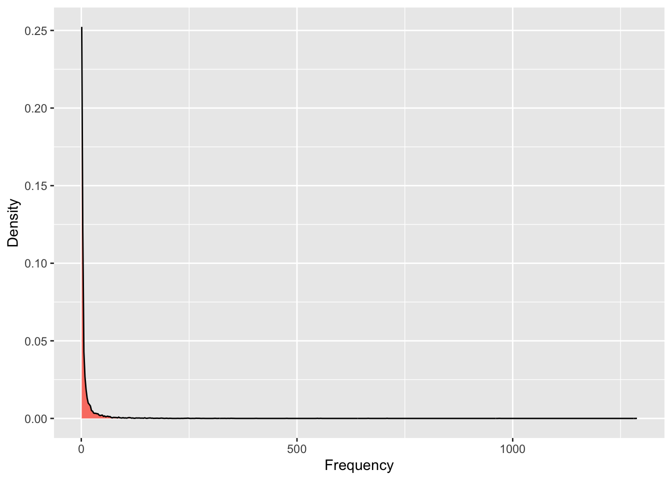

Figure 17.1: Probability density plot of word frequency

A word cloud is way of visualizing the most frequent words.

library(wordcloud)
library(RColorBrewer)
# select the color palette
pal = brewer.pal(5,"Accent")
# generate the cloud based on the 30 most frequent words
wordcloud(d$word, d$freq, min.freq=d$freq[30],colors=pal)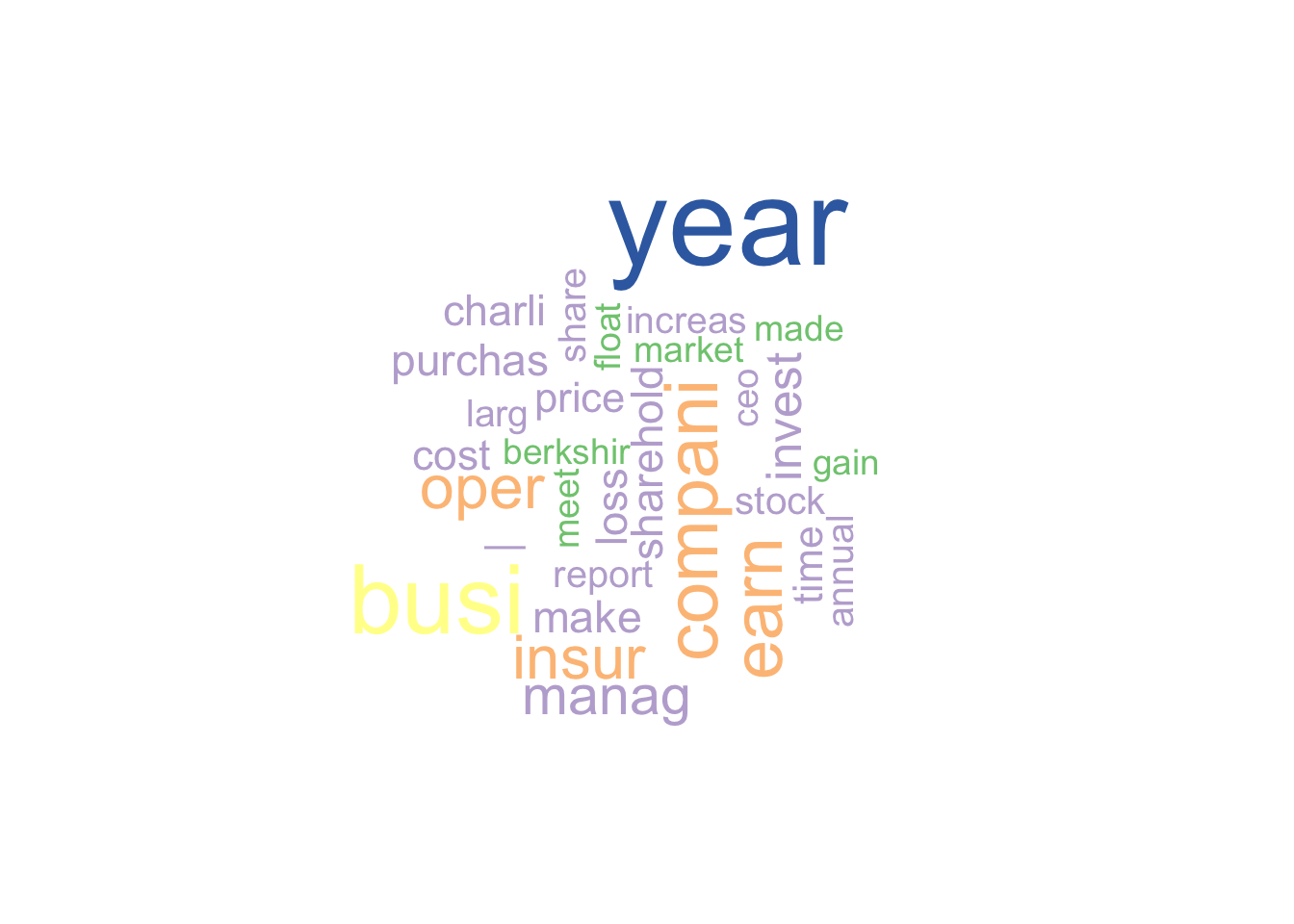

Figure 17.2: A word cloud

❓ Skill builder

Start with the original letters corpus (i.e., prior to preprocessing) and identify the 20 most common words and create a word cloud for these words.

Co-occurrence and association

Co-occurrence measures the frequency with which two words appear together. In the case of document level association, if the two words both appear or neither appears, then the correlation or association is 1. If two words never appear together in the same document, their association is -1.

A simple example illustrates the concept. The following code sets up a corpus of five elementary documents.

library(tm)
data <-  c("word1", "word1 word2","word1 word2 word3","word1 word2 word3 word4","word1 word2 word3 word4 word5")
corpus <-  VCorpus(VectorSource(data))
tdm <-  TermDocumentMatrix(corpus)
as.matrix(tdm)

##        Docs
## Terms   1 2 3 4 5
##   word1 1 1 1 1 1
##   word2 0 1 1 1 1
##   word3 0 0 1 1 1
##   word4 0 0 0 1 1
##   word5 0 0 0 0 1

We compute the correlation of rows to get a measure of association across documents.

# Correlation between word2 and word3, word4, and word5
cor(c(0,1,1,1,1),c(0,0,1,1,1))

## [1] 0.6123724

cor(c(0,1,1,1,1),c(0,0,0,1,1))

## [1] 0.4082483

cor(c(0,1,1,1,1),c(0,0,0,0,1))

## [1] 0.25

Alternatively, use the findAssocs function, which computes all correlations between a given term and all terms in the term-document matrix and reports those higher than the correlation threshold.

library(tm)
# find associations greater than 0.1
findAssocs(tdm,"word2",0.1)

## $word2
## word3 word4 word5 
##  0.61  0.41  0.25

Now that you have an understanding of how association works across documents, here is an example for the corpus of Buffett letters.

# Select the first ten letters
tdm <- TermDocumentMatrix(stem.letters[1:10])
# compute the associations
findAssocs(tdm, "invest",0.80)

## $invest
##      bare     earth imperfect     resum     susan 
##      0.88      0.88      0.88      0.84      0.84

Cluster analysis

Cluster analysis is a statistical technique for grouping together sets of observations that share common characteristics. Objects assigned to the same group are more similar in some way than those allocated to another cluster. In the case of a corpus, cluster analysis groups documents based on their similarity. Google, for instance, uses clustering for its news site.

The general principle of cluster analysis is to map a set of observations in multidimensional space. For example, if you have seven measures for each observation, each will be mapped into seven-dimensional space. Observations that are close together in this space will be grouped together. In the case of a corpus, cluster analysis is based on mapping frequently occurring words into a multidimensional space. The frequency with which each word appears in a document is used as a weight, so that frequently occurring words have more influence than others.

There are multiple statistical techniques for clustering, and multiple methods for calculating the distance between points. Furthermore, the analyst has to decide how many clusters to create. Thus, cluster analysis requires some judgment and experimentation to develop a meaningful set of groups.

The following code computes all possible clusters using the Ward method of cluster analysis. A term-document matrix is sparse, which means it consists mainly of zeroes. In other words, many terms occur in only one or two documents, and the cell entries for the remaining documents are zero. In order to reduce the computations required, sparse terms are removed from the matrix. You can vary the sparse parameter to see how the clusters vary.

# Cluster analysis
# name the columns for the letter's year
tdm <- TermDocumentMatrix(stem.letters[1:15])
colnames(tdm) <-  1998:2012
# Remove sparse terms
tdm1 <- removeSparseTerms(tdm, 0.5)
# transpose the matrix
tdmtranspose <-  t(tdm1)
cluster = hclust(dist(tdmtranspose))
# plot the tree
plot(cluster)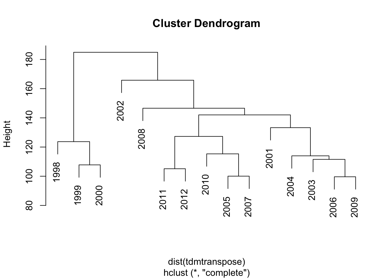

Figure 17.3: Dendrogram for Buffett letters from 1998-2012

The cluster analysis is shown in the following figure as a dendrogram, a tree diagram, with a leaf for each year. Clusters seem to from around consecutive years. Can you think of an explanation?

Topic modeling

Topic modeling is a set of statistical techniques for identifying the themes that occur in a document set. The key assumption is that a document on a particular topic will contain words that identify that topic. For example, a report on gold mining will likely contain words such as “gold” and “ore.” Whereas, a document on France, would likely contain the terms “France,” “French,” and “Paris.”

The package topicmodels implements topic modeling techniques within the R framework. It extends tm to provide support for topic modeling. It implements two methods: latent Dirichlet allocation (LDA), which assumes topics are uncorrelated; and correlated topic models (CTM), an extension of LDA that permits correlation between topics.⁴⁴ Both LDA and CTM require that the number of topics to be extracted is determined a priori. For example, you might decide in advance that five topics gives a reasonable spread and is sufficiently small for the diversity to be understood.⁴⁵

Words that occur frequently in many documents are not good at distinguishing among documents. The weighted term frequency inverse document frequency (tf-idf) is a measure designed for determining which terms discriminate among documents. It is based on the term frequency (tf), defined earlier, and the inverse document frequency.

Inverse document frequency

The inverse document frequency (idf) measures the frequency of a term across documents.

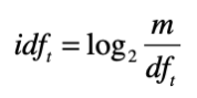
Where m = number of documents (i.e., rows in the case of a term-document matrix); df_t = number of documents containing term t.

If a term occurs in every document, then its idf = 0, whereas if a term occurs in only one document out of 15, its idf = 3.91.

To calculate and display the idf for the letters corpus, we can use the following R script.

# calculate idf for each term
library(slam)
library(ggplot2)
idf <-  log2(nDocs(dtm)/col_sums(dtm > 0))
# create dataframe for graphing
df.idf <-  data.frame(idf)
ggplot(df.idf,aes(idf)) + geom_histogram(fill="chocolate") + xlab("Inverse document frequency")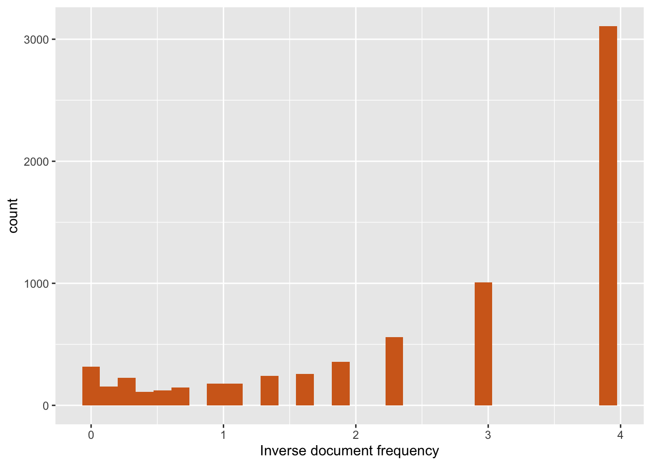

Figure 17.4: Inverse document frequency (corpus has 15 documents)

The generated graphic shows that about 5,000 terms occur in only one document (i.e., the idf = 3.91) and less than 500 terms occur in every document. The terms with an idf in the range 1 to 2 are likely to be the most useful in determining the topic of each document.

Term frequency inverse document frequency (tf-idf)

The weighted term frequency inverse document frequency (tf-idf or ω_td) is calculated by multiplying a term’s frequency (tf) by its inverse document frequency (idf).

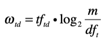
Where tf_td = frequency of term t in document d.

Topic modeling with R

Prior to topic modeling, pre-process a text file in the usual fashion (e.g., convert to lower case, remove punctuation, and so forth). Then, create a document-term matrix.

The mean term frequency-inverse document frequency (tf-idf) is used to select the vocabulary for topic modeling. We use the median value of tf-idf for all terms as a threshold.

library(topicmodels)
library(slam)
# calculate tf-idf for each term
tfidf <-  tapply(dtm$v/row_sums(dtm)[dtm$i], dtm$j, mean) * log2(nDocs(dtm)/col_sums(dtm > 0))
# report dimensions (terms)
dim(tfidf)

## [1] 6966

# report median to use as cut-off point
median(tfidf)

## [1] 0.0006601708

The goal of topic modeling is to find those terms that distinguish a document set. Thus, terms with low frequency should be omitted because they don’t occur often enough to define a topic. Similarly, those terms occurring in many documents don’t differentiate between documents.

A common heuristic is to select those terms with a tf-idf > median(tf-idf). As a result, we reduce the document-term matrix by keeping only those terms above the threshold and eliminating rows that have zero terms. Because the median is a measure of central tendency, this approach reduces the number of columns by roughly half.

# select columns with tf-idf > median
dtm <- dtm[,tfidf >= median(tfidf)]
#select rows with rowsum > 0
dtm <- dtm[row_sums(dtm) > 0,]
# report reduced dimension
dim(dtm)

## [1]   15 3509

As mentioned earlier, the topic modeling method assumes a set number of topics, and it is the responsibility of the analyst to estimate the correct number of topics to extract. It is common practice to fit models with a varying number of topics, and use the various results to establish a good choice for the number of topics. The analyst will typically review the output of several models and make a judgment on which model appears to provide a realistic set of distinct topics. Here is some code that starts with five topics.

# set number of topics to extract
k <- 5 # number of topics
SEED <- 2010 # seed for initializing the model rather than the default random
# try multiple methods – takes a while for a big corpus
TM <- list(VEM = LDA(dtm, k = k, control = list(seed = SEED)),
VEM_fixed = LDA(dtm, k = k, control = list(estimate.alpha = FALSE, seed = SEED)),
Gibbs = LDA(dtm, k = k, method = "Gibbs", control = list(seed = SEED, burnin = 1000,  thin = 100, iter = 1000)), CTM = CTM(dtm, k = k,control = list(seed = SEED, var = list(tol = 10^-3), em = list(tol = 10^-3))))
topics(TM[["VEM"]], 1)

## 1998 1999 2000 2001 2002 2003 2004 2005 2006 2007 2008 2009 2010 2011 2012 
##    2    2    2    3    1    3    3    3    4    3    5    4    1    1    5

terms(TM[["VEM"]], 5)

##      Topic 1     Topic 2     Topic 3   Topic 4   Topic 5     
## [1,] "’"         "—"         "clayton" "walter"  "newspap"   
## [2,] "repurchas" "eja"       "deficit" "clayton" "clayton"   
## [3,] "committe"  "repurchas" "see"     "newspap" "repurchas" 
## [4,] "economi"   "merger"    "member"  "iscar"   "journalist"
## [5,] "bnsf"      "ticket"    "—"       "equita"  "monolin"

The output indicates that the first three letter (1998-2000) are about topic 4, the fourth (2001) topic 2, and so on.

Topic 1 is defined by the following terms: thats, bnsf, cant, blacksholes, and railroad. As we have seen previously, some of these words (e.g., thats and cant, which we can infer as being that’s and can’t) are not useful differentiators, and the dictionary could be extended to remove them from consideration and topic modeling repeated. For this particular case, it might be that Buffett’s letters don’t vary much from year to year, and he returns to the same topics in each annual report.

❓ Skill builder

Experiment with the topicmodels package to identify the topics in Buffett’s > letters. You might need to use the dictionary feature of text mining to remove selected words from the corpus to develop a meaningful distinction between topics.

Named-entity recognition (NER)

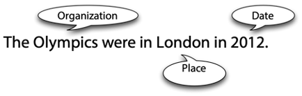
Named-entity recognition (NER) places terms in a corpus into predefined categories such as the names of persons, organizations, locations, expressions of times, quantities, monetary values, and percentages. It identifies some or all mentions of these categories, as shown in the following figure, where an organization, place, and date are recognized.

Named-entity recognition example

Tags are added to the corpus to denote the category of the terms identified.

The Olympics were in London in 2012.

There are two approaches to developing an NER capability. A rules-based approach works well for a well-understood domain, but it requires maintenance and is language dependent. Statistical classifiers, based on machine learning, look at each word in a sentence to decide whether it is the start of a named-entity, a continuation of an already identified named-entity, or not part of a named-entity. Once a named-entity is distinguished, its category (e.g., place) must be identified and surrounding tags inserted.

Statistical classifiers need to be trained on a large collection of human-annotated text that can be used as input to machine learning software. Human-annotation, while time-consuming, does not require a high level of skill. It is the sort of task that is easily parallelized and distributed to a large number of human coders who have a reasonable understanding of the corpus’s context (e.g., able to recognize that London is a place and that the Olympics is an organization). The software classifier need to be trained on approximately 30,000 words.

The accuracy of NER is dependent on the corpus used for training and the domain of the documents to be classified. For example, NER is based on a collection of news stories and is unlikely to be very accurate for recognizing entities in medical or scientific literature. Thus, for some domains, you will likely need to annotate a set of sample documents to create a relevant model. Of course, as times change, it might be necessary to add new annotated text to the learning script to accommodate new organizations, place, people and so forth. A well-trained statistical classifier applied appropriately is usually capable of correctly recognizing entities with 90 percent accuracy.

NER software

OpenNLP is an Apache Java-based machine learning based toolkit for the processing of natural language in text format. It is a collection of natural language processing tools, including a sentence detector, tokenizer, parts-of-speech(POS)-tagger, syntactic parser, and named-entity detector. The NER tool can recognize people, locations, organizations, dates, times. percentages, and money. You will need to write a Java program to take advantage of the toolkit. The R package, openNLP, provides an interface to OpenNLP.

Future developments

Text mining and natural language processing are developing areas and you can expect new tools to emerge. Document summarization, relationship extraction, advanced sentiment analysis, and cross-language information retrieval (e.g., a Chinese speaker querying English documents and getting a Chinese translation of the search and selected documents) are all areas of research that will likely result in generally available software with possible R versions. If you work in this area, you will need to continually scan for new software that extends the power of existing methods and adds new text mining capabilities.

Summary

Language enables cooperation through information exchange. Natural language processing (NLP) focuses on developing and implementing software that enables computers to handle large scale processing of language in a variety of forms, such as written and spoken. The inherent ambiguity in written and spoken speech makes NLP challenging. Don’t expect NLP to provide the same level of exactness and starkness as numeric processing. There are three levels to consider when processing language: semantics, discourse, and pragmatics.

Sentiment analysis is a popular and simple method of measuring aggregate feeling. Tokenization is the process of breaking a document into chunks. A collection of text is called a corpus. The Flesch-Kincaid formula is a common way of assessing readability. Preprocessing, which prepares a corpus for text mining, can include case conversion, punctuation removal, number removal, stripping extra white spaces, stop word filtering, specific word removal, word length filtering, parts of speech (POS) filtering, Stemming, and regex filtering.

Word frequency analysis is a simple technique that can also be the foundation for other analyses. A term-document matrix contains one row for each term and one column for each document. A document-term matrix contains one row for each document and one column for each term. Words that occur frequently within a document are usually a good indicator of the document’s content. A word cloud is way of visualizing the most frequent words. Co-occurrence measures the frequency with which two words appear together. Cluster analysis is a statistical technique for grouping together sets of observations that share common characteristics. Topic modeling is a set of statistical techniques for identifying the topics that occur in a document set. The inverse document frequency (idf) measures the frequency of a term across documents. Named-entity recognition (NER) places terms in a corpus into predefined categories such as the names of persons, organizations, locations, expressions of times, quantities, monetary values, and percentages. Statistical classification is used for NER. OpenNLP is an Apache Java-based machine learning-based toolkit for the processing of natural language in text format. Document summarization, relationship extraction, advanced sentiment analysis, and cross-language information retrieval are all areas of research.

Key terms and concepts

Association	Readability
Cluster analysis	Regex filtering
Co-occurrence	Sentiment analysis
Corpus	Statistical classification
Dendrogram	Stemming
Document-term matrix	Stop word filtering
Flesch-Kincaid formula	Stripping extra white spaces
Inverse document frequency	Term-document matrix
KNIME	Term frequency
Named-entity recognition (NER)	Term frequency inverse document frequency
Natural language processing (NLP)	Text mining
Number removal	Tokenization
OpenNLP	Topic modeling
Parts of speech (POS) filtering	Word cloud
Preprocessing	Word frequency analysis
Punctuation removal	Word length filtering

References

Feinerer, I. (2008). An introduction to text mining in R. R News, 8(2), 19-22.

Feinerer, I., Hornik, K., & Meyer, D. (2008). Text mining infrastructure in R. Journal of Statistical Software, 25(5), 1-54.

Grün, B., & Hornik, K. (2011). topicmodels: An R package for fitting topic models. Journal of Statistical Software, 40(13), 1-30.

Ingersoll, G., Morton, T., & Farris, L. (2012). Taming Text: How to find, organize and manipulate it. Greenwich, CT: Manning Publications.

Exercises

Take the recent annual reports for UPS and convert them to text using an online service, such as.

Complete the following tasks:
1. Count the words in the most recent annual report.
2. Compute the readability of the most recent annual report.
3. Create a corpus.
4. Preprocess the corpus.
5. Create a term-document matrix and compute the frequency of words in the corpus.
6. Construct a word cloud for the 25 most common words.
7. Undertake a cluster analysis, identify which reports are similar in nature, and see if you can explain why some reports are in different clusters.
8. Build a topic model for the annual reports.
Merge the annual reports for Berkshire Hathaway (i.e., Buffett’s letters) and UPS into a single corpus.
1. Undertake a cluster analysis and identify which reports are similar in nature.
2. Build a topic model for the combined annual reports.
3. Do the cluster analysis and topic model suggest considerable differences in the two sets of reports?

Ambiguities are often the inspiration for puns. “You can tune a guitar, but you can’t tuna fish. Unless of course, you play bass,” by Douglas Adams↩︎
The mathematics of LDA and CTM are beyond the scope of this text. For details, see Grün, B., & Hornik, K. (2011). Topicmodels: An R package for fitting topic models. Journal of Statistical Software, 40(13), 1-30. ↩︎
Humans have a capacity to handle about 7±2 concepts at a time. Miller, G. A. (1956). The magical number seven, plus or minus two: some limits on our capacity for processing information. The Psychological Review, 63(2), 81-97. ↩︎