Chapter 14 Organizational Intelligence
There are three kinds of intelligence: One kind understands things for itself, the other appreciates what others can understand, the third understands neither for itself nor through others. This first kind is excellent, the second good, and the third kind useless.
Machiavelli, The Prince, 1513
Learning objectives
Students completing this chapter will be able to
understand the principles of organizational intelligence;
decide whether to use verification or discovery for a given problem;
select the appropriate data analysis technique(s) for a given situation;
Information poverty
Too many companies are data rich but information poor. They collect vast amounts of data with their transaction processing systems, but they fail to turn these data into the necessary information to support managerial decision making. Many organizations make limited use of their data because they are scattered across many systems rather than centralized in one readily accessible, integrated data store. Technologies exist to enable organizations to create vast repositories of data that can be then analyzed to inform decision making and enhance operational performance.
Organizational intelligence is the outcome of an organization’s efforts to collect, store, process, and interpret data from internal and external sources. The conclusions or clues gleaned from an organization’s data stores enable it to identify problems or opportunities, which is the first stage of decision making.
An organizational intelligence system
Transaction processing systems (TPSs) are a core component of organizational memory and thus an important source of data. Along with relevant external information, the various TPSs are the bedrock of an organizational intelligence system. They provide the raw facts that an organization can use to learn about itself, its competitors, and the environment. A TPS can generate huge volumes of data. In the United States, a telephone company may generate millions of records per day detailing the telephone calls it has handled. The hundreds of million credit cards on issue in the world generate billions of transactions per year. A popular Web site can have a hundred million hits per day. TPSs are creating a massive torrent of data that potentially reveals to an organization a great deal about its business and its customers.
Unfortunately, many organizations are unable to exploit, either effectively or efficiently, the massive amount of data generated by TPSs. Data are typically scattered across a variety of systems, in different database technologies, in different operating systems, and in different locations. The fundamental problem is that organizational memory is fragmented. Consequently, organizations need a technology that can accumulate a considerable proportion of organizational memory into one readily accessible system. Making these data available to decision makers is crucial to improving organizational performance, providing first-class customer service, increasing revenues, cutting costs, and preparing for the future. For many organizations, their memory is a major untapped resource—an underused intelligence system containing undetected key facts about customers. To take advantage of the mass of available raw data, an organization first needs to organize these data into one logical collection and then use software to sift through this collection to extract meaning.
The data warehouse or a data lake, a subject-oriented, integrated, time-variant, and nonvolatile set of data that supports decision making, is a key mean for harnessing organizational memory. Subject databases are designed around the essential entities of a business (e.g., customer) rather than applications (e.g., auto insurance). Integrated implies consistency in naming conventions, keys, relationships, encoding, and translation (e.g., gender is coded consistently across all relevant fields). Time-variant means that data are organized by various time periods (e.g., by months). Because a data warehouse is updated with a bulk upload, rather than as transactions occur, it contains nonvolatile data.
Data warehouses are enormous collections of data, often measured in petabytes, compiled by mass marketers, retailers, and service companies from the transactions of their millions of customers. Associated with a data warehouse are data management aids (e.g., data extraction), analysis tools (e.g., OLAP), and applications (e.g., executive information system).
The data warehouse
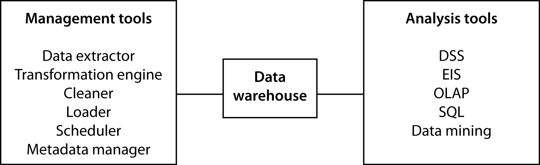
The data warehouse
Creating and maintaining the data warehouse
A data warehouse is a snapshot of an organization at a particular time. In order to create this snapshot, data must be extracted from existing systems, transformed, cleaned, and loaded into the data warehouse. In addition, regular snapshots must be taken to maintain the usefulness of the warehouse.
Extraction
Data from the operational systems, stored in operational data stores (ODS), are the raw material of a data warehouse. Unfortunately, it is not simply a case of pulling data out of ODSs and loading them into the warehouse. Operational systems were often written many years ago at different times. There was no plan to merge these data into a single system. Each application is independent or shares little data with others. The same data may exist in different systems with different names and in different formats. The extraction of data from many different systems is time-consuming and complex. Furthermore, extraction is not a one-time process. Data must be extracted from operational systems on an ongoing basis so that analysts can work with current data.
Transformation
Transformation is part of the data extraction process. In the warehouse, data must be standardized and follow consistent coding systems. There are several types of transformation:
Encoding: Non-numeric attributes must be converted to a common coding system. Gender may be coded, for instance, in a variety of ways (e.g., m/f, 1/0, or M/F) in different systems, and do not take account of social changes that recognize other categories. The extraction program must transform data from each application to a single coding system (e.g., m/f/…).
Unit of measure: Distance, volume, and weight can be recorded in varying units in different systems (e.g., centimeters or inches) and must be converted to a common system.
Field: The same attribute may have different names in different applications (e.g., sales-date, sdate, or saledate), and a standard name must be defined.
Date: Dates could be stored in a variety of ways. In Europe the standard for date is dd/mm/yy, in the U.S. it is mm/dd/yy, whereas the ISO standard is yyyy-mm-dd.
Cleaning
Unfortunately, some of the data collected from applications may be dirty—they contain errors, inconsistencies, or redundancies. There are a variety of reasons why data may need cleaning:
The same record is stored by several departments. For instance, both Human Resources and Production have an employee record. Duplicate records must be deleted.
Multiple records for a company exist because of an acquisition. For example, the record for Sun Microsystems should be removed because it was acquired by Oracle.
Multiple entries for the same entity exist because there are no corporate data entry standards. For example, FedEx and Federal Express both appear in different records for the same company.
Data entry fields are misused. For example, an address line field is used to record a second phone number.
Data cleaning starts with determining the dirtiness of the data. An analysis of a sample should indicate the extent of the problem and whether commercial data-cleaning tools are required. Data cleaning is unlikely to be a one-time process. All data added to the data warehouse should be validated in order to maintain the integrity of the warehouse. Cleaning can be performed using specialized software or custom-written code.
Loading
Data that have been extracted, transformed, and cleaned can be loaded into the warehouse. There are three types of data loads:
Archival: Historical data (e.g., sales for the period 2011–2021) that is loaded once. Many organizations may elect not to load these data because of their low value relative to the cost of loading.
Current: Data from current operational systems.
Ongoing: Continual revision of the warehouse as operational data are generated. Managing the ongoing loading of data is the largest challenge for warehouse management. This loading is done either by completely reloading the data warehouse or by just updating it with the changes.
Scheduling
Refreshing the warehouse, which can take many hours, must be scheduled as part of a data center’s regular operations. Because a data warehouse supports medium- to long-term decision making, it is unlikely that it would need to be refreshed more frequently than daily. For shorter decisions, operational systems are available. Some firms may decide to schedule less frequently after comparing the cost of each load with the cost of using data that are a few days old.
Metadata
A data dictionary is a reference repository containing metadata (i.e., data about data). It includes a description of each data type, its format, coding standards (e.g., volume in liters), and the meaning of the field. For the data warehouse setting, a data dictionary is likely to include details of which operational system created the data, transformations of the data, and the frequency of extracts. Analysts need access to metadata so that they can plan their analyses and learn about the contents of the data warehouse. If a data dictionary does not exist, it should be established and maintained as part of ensuring the integrity of the data warehouse.
Data warehouse technology
Selecting an appropriate data warehouse system is critical to support significant data analytics. Data analysis often requires intensive processing of large volumes of data, and large main memories are necessary for good performance. In addition, the system should be scalable so that as the demand for data analysis grows, the system can be readily upgraded.
Some organizations use Hadoop, which is covered in the chapter on cluster computing, as the foundation for a data warehouse. It offers speed and cost advantages over prior technology .
Exploiting data stores
Two approaches to analyzing a data store (i.e., a database or data warehouse) are data mining and data analytics. Before discussing each of these approaches, it is helpful to recognize the fundamentally different approaches that can be taken to exploiting a data store.
Verification and discovery
The verification approach to data analysis is driven by a hypothesis or conjecture about some relationship (e.g., customers with incomes in the range of $50,000–75,000 are more likely to buy minivans). The analyst then formulates a query to process the data to test the hypothesis. The resulting report will either support or disconfirm the theory. If the theory is disconfirmed, the analyst may continue to propose and test hypotheses until a target customer group of likely prospects for minivans is identified. Then, the minivan firm may market directly to this group because the likelihood of converting them to customers is higher than mass marketing to everyone. The verification approach is highly dependent on a persistent analyst eventually finding a useful relationship (i.e., who buys minivans?) by testing many hypotheses. Statistical methods support the verification approach.
Data mining uses the discovery approach. It sifts through the data in search of frequently occurring patterns and trends to report generalizations about the data. Data mining tools operate with minimal guidance from the client. They are designed to yield useful facts about business relationships efficiently from a large data store. The advantage of discovery is that it may uncover important relationships that no amount of conjecturing would have revealed and tested. Machine learning is a popular discovery tool when large volumes observations are available.
A useful analogy for thinking about the difference between verification and discovery is the difference between conventional and open-pit gold mining. A conventional mine is worked by digging shafts and tunnels with the intention of intersecting the richest gold vein. Verification is like conventional mining—some parts of the gold deposit may never be examined. The company drills where it believes there will be gold. In open-pit mining, everything is excavated and processed. Discovery is similar to open-pit mining—everything is examined. Both verification and discovery are useful; it is not a case of selecting one or the other. Indeed, analysts should use both methods to gain as many insights as possible from the data.
Comparison of verification and discovery
| Verification | Discovery |
|---|---|
| What is the average sale for in-store and catalog customers? | What is the best predictor of sales? |
| What is the average high school GPA of students who graduate from college compared to those who do not? | What are the best predictors of college graduation? |
OLAP
Edgar F. Codd, the father of the relational model, and some colleagues34 proclaimed in 1993 that RDBMSs were never intended to provide powerful functions for data synthesis, analysis, and consolidation. This was the role of spreadsheets and special-purpose applications. He argued that analysts need data analysis tools that complement RDBMS technology, and they put forward the concept of online analytical processing (OLAP): the analysis of business operations with the intention of making timely and accurate analysis-based decisions.
Instead of rows and columns, OLAP tools provide multidimensional views of data, as well as some other differences. OLAP means fast and flexible access to large volumes of derived data whose underlying inputs may be changing continuously.
Comparison of TPS and OLAP applications
| TPS | OLAP |
|---|---|
| Optimized for transaction volume | Optimized for data analysis |
| Process a few records at a time | Process summarized data |
| Real-time update as transactions occur | Batch update (e.g., daily) |
| Based on tables | Based on hypercubes |
| Raw data | Aggregated data |
| SQL | MDX |
For instance, an OLAP tool enables an analyst to view how many widgets were shipped to each region by each quarter in 2012. If shipments to a particular region are below budget, the analyst can find out which customers in that region are ordering less than expected. The analyst may even go as far as examining the data for a particular quarter or shipment. As this example demonstrates, the idea of OLAP is to give analysts the power to view data in a variety of ways at different levels. In the process of investigating data anomalies, the analyst may discover new relationships. The operations supported by the typical OLAP tool include
Calculations and modeling across dimensions, through hierarchies, or across members
Trend analysis over sequential time periods
Slicing subsets for on-screen viewing
Drill-down to deeper levels of consolidation
Drill-through to underlying detail data
Rotation to new dimensional comparisons in the viewing area
An OLAP system should give fast, flexible, shared access to analytical information. Rapid access and calculation are required if analysts are to make ad hoc queries and follow a trail of analysis. Such quick-fire analysis requires computational speed and fast access to data. It also requires powerful analytic capabilities to aggregate and order data (e.g., summarizing sales by region, ordered from most to least profitable). Flexibility is another desired feature. Data should be viewable from a variety of dimensions, and a range of analyses should be supported.
Multidimensional database (MDDB)
OLAP is typically used with an multidimensional database (MDDB), a data management system in which data are represented by a multidimensional structure. The MDDB approach is to mirror and extend some of the features found in spreadsheets by moving beyond two dimensions. These tools are built directly into the MDDB to increase the speed with which data can be retrieved and manipulated. These additional processing abilities, however, come at a cost. The dimensions of analysis must be identified prior to building the database. In addition, MDDBs have size limitations that RDBMSs do not have and, in general, are an order of magnitude smaller than a RDBMS.
MDDB technology is optimized for analysis, whereas relational technology is optimized for the high transaction volumes of a TPS. For example, SQL queries to create summaries of product sales by region, region sales by product, and so on, could involve retrieving many of the records in a marketing database and could take hours of processing. A MDDB could handle these queries in a few seconds. TPS applications tend to process a few records at a time (e.g., processing a customer order may entail one update to the customer record, two or three updates to inventory, and the creation of an order record). In contrast, OLAP applications usually deal with summarized data.
Fortunately, RDBMS vendors have standardized on SQL, and this provides a commonality that allows analysts to transfer considerable expertise from one relational system to another. Similarly, MDX, originally developed by Microsoft to support multidimensional querying of an SQL server, has been implemented by a number of vendors for interrogating an MDDB.
The current limit of MDDB technology is approximately 10 dimensions, which can be millions to trillions of data points.
ROLAP
An alternative to a physical MDDB is a relational OLAP (or ROLAP), in which case a multidimensional model is imposed on a relational model. As we discussed earlier, this is also known as a logical MDDB. Not surprisingly, a system designed to support OLAP should be superior to trying to retrofit relational technology to a task for which it was not specifically designed.
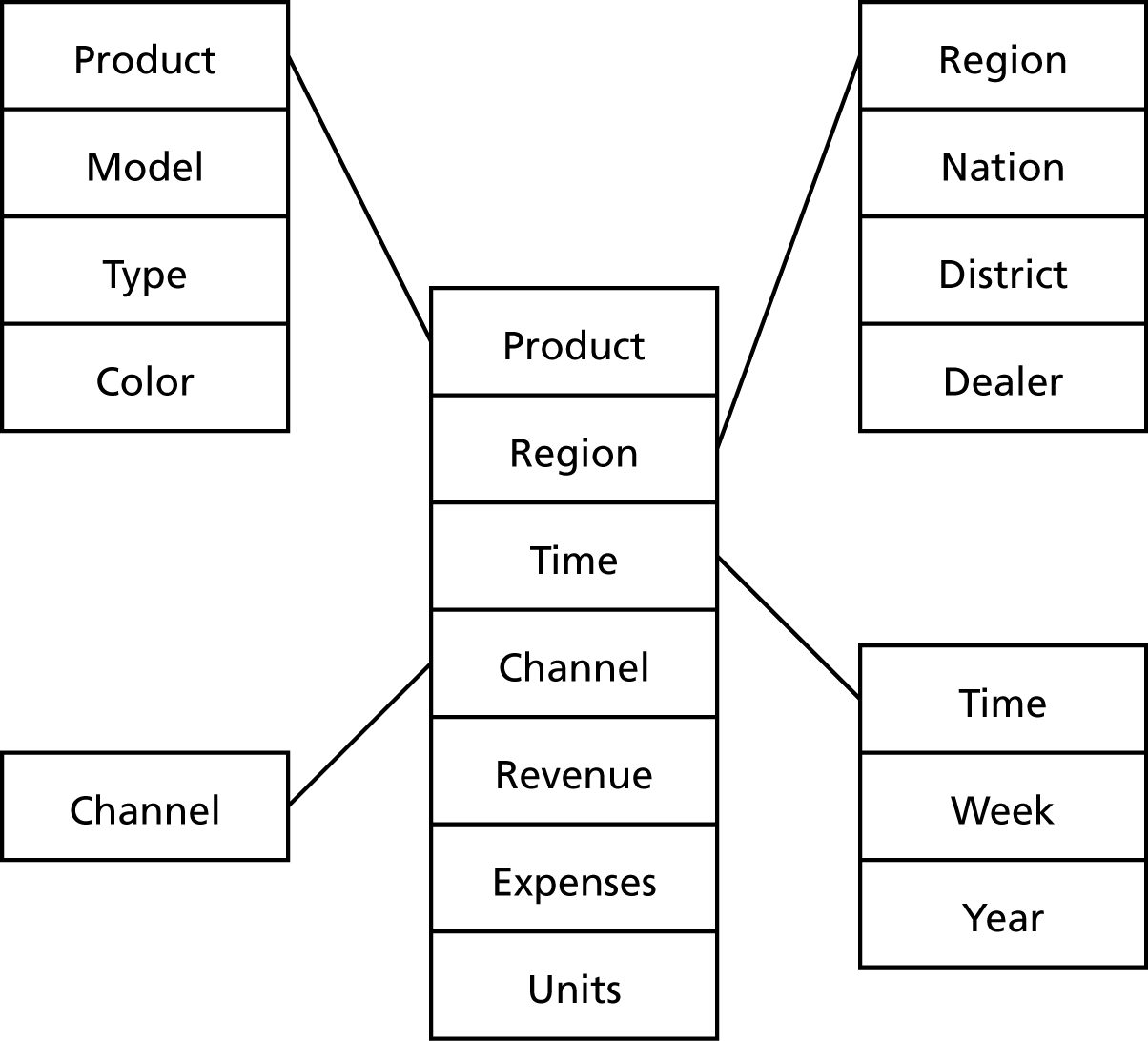
The star schema is used by some MDDBs to represent multidimensional data within a relational structure. The center of the star is a table storing multidimensional facts derived from other tables. Linked to this central table are the dimensions (e.g., region) using the familiar primary-key/foreign-key approach of the relational model. The following figure depicts a star schema for an international automotive company. The advantage of the star model is that it makes use of a RDBMS, a mature technology capable of handling massive data stores and having extensive data management features (e.g., backup and recovery). However, if the fact table is very large, which is often the case, performance may be slow. A typical query is a join between the fact table and some of the dimensional tables.
A star schema
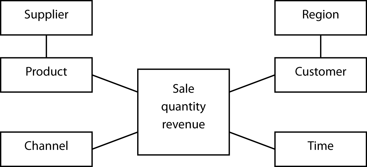
A snowflake schema, more complex than a star schema, resembles a snowflake. Dimensional data are grouped into multiple tables instead of one large table. Space is saved at the expense of query performance because more joins must be executed. Unless you have good reasons, you should opt for a star over a snowflake schema.
A snowflake schema
Rotation, drill-down, and drill-through
MDDB technology supports rotation of data objects (e.g., changing the view of the data from “by year” to “by region” as shown in the following figure) and drill-down (e.g., reporting the details for each nation in a selected region as shown in the Drill Down figure), which is also possible with a relational system. Drill-down can slice through several layers of summary data to get to finer levels of detail. The Japanese data, for instance, could be dissected by region (e.g., Tokyo), and if the analyst wants to go further, Tokyo could be analyzed by store. In some systems, an analyst can drill through the summarized data to examine the source data within the organizational data store from which the MDDB summary data were extracted.
Rotation
| Region | |||||
|---|---|---|---|---|---|
| Year | Data | Asia | Europe | North America | Grand total |
| 2010 | Sum of hardware | 97 | 23 | 198 | 318 |
| Sum of software | 83 | 41 | 425 | 549 | |
| 2011 | Sum of hardware | 115 | 28 | 224 | 367 |
| Sum of software | 78 | 65 | 410 | 553 | |
| 2012 | Sum of hardware | 102 | 25 | 259 | 386 |
| Sum of software | 55 | 73 | 497 | 625 | |
| Total sum of hardware | 314 | 76 | 681 | 1,071 | |
| Total sum of software | 216 | 179 | 1,322 | 1717 |
Global regional results
| Region | Sales variance (^) |
|---|---|
| Africa | 105 |
| Asia | 57 |
| Europe | 122 |
| North America | 97 |
| Pacific | 85 |
| South America | 163 |
Asia drilldown | Nation | Sales variance (%) | |:———-|—————-:| | China | 123 | | Japan | 52 | | India | 87 | | Singapore | 95 |
The hypercube
From the analyst’s perspective, a fundamental difference between MDDB and RDBMS is the representation of data. As you know from data modeling, the relational model is based on tables, and analysts must think in terms of tables when they manipulate and view data. The relational world is two-dimensional. In contrast, the hypercube is the fundamental representational unit of a MDDB. Analysts can move beyond two dimensions. To envisage this change, consider the difference between the two-dimensional blueprints of a house and a three-dimensional model. The additional dimension provides greater insight into the final form of the building.
A hypercube

Of course, on a screen or paper only two dimensions can be shown. This problem is typically overcome by selecting an attribute of one dimension (e.g., North region) and showing the other two dimensions (i.e., product sales by year). You can think of the third dimension (i.e., region in this case) as the page dimension—each page of the screen shows one region or slice of the cube.
| Page | Columns | |||
|---|---|---|---|---|
| Region: North | Sales | |||
| Red blob | Blue blob | Total | ||
| 2011 | ||||
| Rows | 2012 | |||
| Year | Total |
A three-dimensional hypercube display
A hypercube can have many dimensions. Consider the case of a furniture retailer who wants to capture six dimensions of data. Although it is extremely difficult to visualize a six-dimensional hypercube, it helps to think of each cell of the cube as representing a fact (e.g., the Atlanta store sold five Mt. Airy desks to a business in January).
A six-dimensional hypercube
| Dimension | Example |
|---|---|
| Brand | Mt. Airy |
| Store | Atlanta |
| Customer segment | Business |
| Product group | Desks |
| Period | January |
| Variable | Units sold |
Similarly, a six-dimensional hypercube can be represented by combining dimensions (e.g., brand and store can be combined in the row dimension by showing stores within a brand).
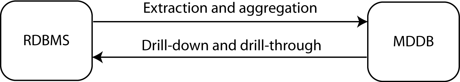
A quick inspection of the table of the comparison of TPS and OLAP applications reveals that relational and multidimensional database technologies are designed for very different circumstances. Thus, the two technologies should be considered as complementary, not competing, technologies. Appropriate data can be periodically extracted from an RDBMS, aggregated, and loaded into an MDDB. Ideally, this process is automated so that the MDDB is continuously updated. Because analysts sometimes want to drill down to low-level aggregations and even drill through to raw data, there must be a connection from the MDDB to the RDBMS to facilitate access to data stored in the relational system.
The relationship between RDBMS and MDDB
Designing a multidimensional database
The multidimensional model, based on the hypercube, requires a different design methodology from the relational model. At this stage, there is no commonly used approach, such as the entity-relationship principle of the relational model. However, the method proposed by Thomsen 35 deserves consideration.
The starting point is to identify what must be tracked (e.g., sales for a retailer or revenue per passenger mile for a transportation firm). A collection of tracking variables is called a variable dimension.
The next step is to consider what types of analyses will be performed on the variable dimension. In a sales system, these may include sales by store by month, comparison of this month’s sales with last month’s for each product, and sales by class of customer. These types of analyses cannot be conducted unless the instances of each variable have an identifying tag. In this case, each sale must be tagged with time, store, product, and customer type. Each set of identifying factors is an identifier dimension. As a cross-check for identifying either type of dimension, use these six basic prompts.
Basic prompts for determining dimensions
| Prompt | Example | Source |
|---|---|---|
| When? | June 5, 2013 10:27am | Transaction data |
| Where? | Paris | |
| What? | Tent | |
| How? | Catalog | |
| Who? | Young adult woman | Face recognition or credit card issuer |
| Why? | Camping trip to Bolivia | Social media |
| Outcome? | Revenue of €624.00 | Transaction data |
Most of the data related to the prompts can be extracted from transactional data. Face recognition software could be used to estimate the age and gender of the buyer in a traditional retail establishment. If the buyer uses a credit card, then such data, with greater precision, could be obtained from the bank issuing the credit card. In the case of why, the motivation for the purchase, the retailer can mine social exchanges made by the customer. Of course, this requires the retailer to be able to uniquely identify the buyer, through a store account or credit card, and use this identification to mine social media.
Variables and identifiers are the key concepts of MDDB design. The difference between the two is illustrated in the following table. Observe that time, an identifier, follows a regular pattern, whereas sales do not. Identifiers are typically known in advance and remain constant (e.g., store name and customer type), while variables change. It is this difference that readily distinguishes between variables and identifiers. Unfortunately, when this is not the case, there is no objective method of discriminating between the two. As a result, some dimensions can be used as both identifiers and variables.
A sales table
| Identifier (time) | Variable sales (dollars) |
|---|---|
| 10:00 | 523 |
| 11:00 | 789 |
| 12:00 | 1,256 |
| 13:00 | 4,128 |
| 14:00 | 2,634 |
+—————-+—————–+
There can be a situation when your intuitive notion of an identifier and variable is not initially correct. Consider a Web site that is counting the number of hits on a particular page. In this case, the identifier is hit and time is the variable because the time of each hit is recorded.
A hit table
| Identifier (hit) | Variable (time) |
|---|---|
| 1 | 9:34:45 |
| 2 | 9:34:57 |
| 3 | 9:36:12 |
| 4 | 9:41:56 |
The next design step is to consider the form of the dimensions. You will recall from statistics that there are three types of variables (dimensions in MDDB language): nominal, ordinal, and continuous. A nominal variable is an unordered category (e.g., region), an ordinal variable is an ordered category (e.g., age group), and a continuous variable has a numeric value (e.g., passenger miles). A hypercube is typically a combination of several types of dimensions. For instance, the identifier dimensions could be product and store (both nominal), and the variable dimensions could be sales and customers. A dimension’s type comes into play when analyzing relationships between identifiers and variables, which are known as independent and dependent variables in statistics. The most powerful forms of analysis are available when both dimensions are continuous. Furthermore, it is always possible to recode a continuous variable into ordinal categories. As a result, wherever feasible, data should be collected as a continuous dimension.
Relationship of dimension type to possible analyses
| Identifier dimension | |||
|---|---|---|---|
| Continuous | Nominal or ordinal | ||
| Variable dimension | Continuous | Regression and curve fitting | Analysis of variance |
| Sales over time | Sales by store | ||
| Nominal or ordinal | Logistic regression | Contingency table analysis | |
| Customer response (yes or no) to the level of advertisng | Number of sales by region |
This brief introduction to multidimensionality modeling has demonstrated the importance of distinguishing between types of dimensions and considering how the form of a dimension (e.g., nominal or continuous) will affect the choice of analysis tools. Because multidimensional modeling is a relatively new concept, you can expect design concepts to evolve. If you become involved in designing an MDDB, then be sure to review carefully current design concepts. In addition, it would be wise to build some prototype systems, preferably with different vendor implementations of the multidimensional concept, to enable analysts to test the usefulness of your design.
❓ Skill builder
A national cinema chain has commissioned you to design a multidimensional database for its marketing department. What identifier and variable dimensions would you select?
Data mining
Data mining is the search for relationships and global patterns that exist in large databases but are hidden in the vast amounts of data. In data mining, an analyst combines knowledge of the data with advanced machine learning technologies to discover nuggets of knowledge hidden in the data. Data mining software can find meaningful relationships that might take years to find with conventional techniques. The software is designed to sift through large collections of data and, by using statistical and artificial intelligence techniques, identify hidden relationships. The mined data typically include electronic point-of-sale records, inventory, customer transactions, and customer records with matching demographics, usually obtained from an external source. Data mining does not require the presence of a data warehouse. An organization can mine data from its operational files or independent databases. However, data mining independent files will not uncover relationships that exist between data in different files. Data mining will usually be easier and more effective when the organization accumulates as much data as possible in a single data store, such as a data warehouse. Recent advances in processing speeds and lower storage costs have made large-scale mining of corporate data a reality.
Database marketing, a common application of data mining, is also one of the best examples of the effective use of the technology. Database marketers use data mining to develop, test, implement, measure, and modify tailored marketing programs. The intention is to use data to maintain a lifelong relationship with a customer. The database marketer wants to anticipate and fulfill the customer’s needs as they emerge. For example, recognizing that a customer buys a new car every three or four years and with each purchase gets an increasingly more luxurious car, the car dealer contacts the customer during the third year of the life of the current car with a special offer on its latest luxury model.
Data mining uses
There are many applications of data mining:
Predicting the probability of default for consumer loan applications. Data mining can help lenders reduce loan losses substantially by improving their ability to predict bad loans.
Reducing fabrication flaws in VLSI chips. Data mining systems can sift through vast quantities of data collected during the semiconductor fabrication process to identify conditions that cause yield problems.
Predicting audience share for television programs. A market-share prediction system allows television programming executives to arrange show schedules to maximize market share and increase advertising revenues.
Predicting the probability that a cancer patient will respond to radiation therapy. By more accurately predicting the effectiveness of expensive medical procedures, health care costs can be reduced without affecting quality of care.
Predicting the probability that an offshore oil well is going to produce oil. An offshore oil well may cost $30 million. Data mining technology can increase the probability that this investment will be profitable.
Identifying quasars from trillions of bytes of satellite data. This was one of the earliest applications of data mining systems, because the technology was first applied in the scientific community.
Data mining functions
Based on the functions they perform, five types of data mining functions exist:
Associations
An association function identifies affinities existing among the collection of items in a given set of records. These relationships can be expressed by rules such as “72 percent of all the records that contain items A, B, and C also contain items D and E.” Knowing that 85 percent of customers who buy a certain brand of wine also buy a certain type of pasta can help supermarkets improve use of shelf space and promotional offers. Discovering that fathers, on the way home on Friday, often grab a six-pack of beer after buying some diapers, enabled a supermarket to improve sales by placing beer specials next to diapers.
Sequential patterns
Sequential pattern mining functions identify frequently occurring sequences from given records. For example, these functions can be used to detect the set of customers associated with certain frequent buying patterns. Data mining might discover, for example, that 32 percent of female customers within six months of ordering a red jacket also buy a gray skirt. A retailer with knowledge of this sequential pattern can then offer the red-jacket buyer a coupon or other enticement to attract the prospective gray-skirt buyer.
Classifying
Classifying divides predefined classes (e.g., types of customers) into mutually exclusive groups, such that the members of each group are as close as possible to one another, and different groups are as far as possible from one another, where distance is measured with respect to specific predefined variables. The classification of groups is done before data analysis. Thus, based on sales, customers may be first categorized as infrequent, occasional, and frequent. ***A classifier could be used to identify those attributes, from a given set, that discriminate among the three types of customers. For example, a classifier might identify frequent customers as those with incomes above $50,000 and having two or more children. Classification functions have been used extensively in applications such as credit risk analysis, portfolio selection, health risk analysis, and image and speech recognition. Thus, when a new customer is recruited, the firm can use the classifying function to determine the customer’s sales potential and accordingly tailor its market to that person.
Clustering
Whereas classifying starts with predefined categories, clustering starts with just the data and discovers the hidden categories. These categories are derived from the data. Clustering divides a dataset into mutually exclusive groups such that the members of each group are as close as possible to one another, and different groups are as far as possible from one another, where distance is measured with respect to all available variables. The goal of clustering is to identify categories. Clustering could be used, for instance, to identify natural groupings of customers by processing all the available data on them. Examples of applications that can use clustering functions are market segmentation, discovering affinity groups, and defect analysis.
Prediction
Prediction calculates the future value of a variable. For example, it might be used to predict the revenue value of a new customer based on that person’s demographic variables.
These various data mining techniques can be used together. For example, a sequence pattern analysis could identify potential customers (e.g., red jacket leads to gray skirt), and then classifying could be used to distinguish between those prospects who are converted to customers and those who are not (i.e., did not follow the sequential pattern of buying a gray skirt). This additional analysis should enable the retailer to refine its marketing strategy further to increase the conversion rate of red-jacket customers to gray-skirt purchasers.
Data mining technologies
Data miners use technologies that are based on statistical analysis and data visualization.
Decision trees
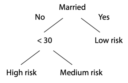
Tree-shaped structures can be used to represent decisions and rules for the classification of a dataset. As well as being easy to understand, tree-based models are suited to selecting important variables and are best when many of the predictors are irrelevant. A decision tree, for example, can be used to assess the risk of a prospective renter of an apartment.
A decision tree
Genetic algorithms
Genetic algorithms are optimization techniques based on the concepts of biological evolution, and use processes such as genetic combination, mutation, and natural selection. Possible solutions for a problem compete with each other. In an evolutionary struggle of the survival of the fittest, the best solution survives the battle. Genetic algorithms are suited for optimization problems with many candidate variables (e.g., candidates for a loan).
K-nearest-neighbor method
The nearest-neighbor method is used for clustering and classification. In the case of clustering, the method first plots each record in n-dimensional space, where n attributes are used in the analysis. Then, it adjusts the weights for each dimension to cluster together data points with similar goal features. For instance, if the goal is to identify customers who frequently switch phone companies, the k-nearest-neighbor method would adjust weights for relevant variables (such as monthly phone bill and percentage of non-U.S. calls) to cluster switching customers in the same neighborhood. Customers who did not switch would be clustered some distance apart.
Neural networks
A neural network, mimicking the neurophysiology of the human brain, can learn from examples to find patterns in data and classify data. Although neural networks can be used for classification, they must first be trained to recognize patterns in a sample dataset. Once trained, a neural network can make predictions from new data. Neural networks are suited to combining information from many predictor variables; they work well when many of the predictors are partially redundant. One shortcoming of a neural network is that it can be viewed as a black box with no explanation of the results provided. Often managers are reluctant to apply models they do not understand, and this can limit the applicability of neural networks.
Data visualization
Data visualization can make it possible for the analyst to gain a deeper, intuitive understanding of data. Because they present data in a visual format, visualization tools take advantage of our capability to discern visual patterns rapidly. Data mining can enable the analyst to focus attention on important patterns and trends and explore these in depth using visualization techniques. Data mining and data visualization work especially well together.
SQL-99 and OLAP
SQL-99 includes extensions to the GROUP BY clause to support some of the data aggregation capabilities typically required for OLAP. Prior to SQL-99, the following questions required separate queries:
Find the total revenue.
Report revenue by location.
Report revenue by channel.
Report revenue by location and channel.
❓Skill builder
Write SQL to answer each of the four preceding queries using the exped table, which is a sample of 1,000 sales transactions for a retailer.
Writing separate queries is time-consuming for the analyst and is inefficient because it requires multiple passes of the table. SQL-99 introduced GROUPING SETS, ROLLUP, and CUBE as a means of getting multiple answers from a single query and addressing some of the aggregation requirements necessary for OLAP.
Grouping sets
The GROUPING SETS clause is used to specify multiple aggregations in a single query and can be used with all the SQL aggregate functions. In the following SQL statement, aggregations by location and channel are computed. In effect, it combines questions 2 and 3 of the preceding list.
| location | channel | revenue |
|---|---|---|
| null | Catalog | 108762 |
| null | Store | 347537 |
| null | Web | 27166 |
| London | null | 214334 |
| New York | null | 39123 |
| Paris | null | 143303 |
| Sydney | null | 29989 |
| Tokyo | null | 56716 |
The query sums revenue by channel or location. The null in a cell implies that there is no associated location or channel value. Thus, the total revenue for catalog sales is 108,762, and that for Tokyo sales is 56,716.
Although GROUPING SETS enables multiple aggregations to be written as a single query, the resulting output is hardly elegant. It is not a relational table, and thus a view based on GROUPING SETS should not be used as a basis for further SQL queries.
Rollup
The ROLLUP option supports aggregation across multiple columns. It can be used, for example, to cross-tabulate revenue by channel and location.
| location | channel | revenue |
|---|---|---|
| null | null | 483465 |
| London | null | 214334 |
| New York | null | 39123 |
| Paris | null | 143303 |
| Sydney | null | 29989 |
| Tokyo | null | 56716 |
| London | Catalog | 50310 |
| London | Store | 151015 |
| London | Web | 13009 |
| New York | Catalog | 8712 |
| New York | Store | 28060 |
| New York | Web | 2351 |
| Paris | Catalog | 32166 |
| Paris | Store | 104083 |
| Paris | Web | 7054 |
| Sydney | Catalog | 5471 |
| Sydney | Store | 21769 |
| Sydney | Web | 2749 |
| Tokyo | Catalog | 12103 |
| Tokyo | Store | 42610 |
| Tokyo | Web | 2003 |
In the columns with null for location and channel, the preceding query reports a total revenue of 483,465. It also reports the total revenue for each location and revenue for each combination of location and channel. For example, Tokyo Web revenue totaled 2,003.
Cube
CUBE reports all possible values for a set of reporting variables. If SUM is used as the aggregating function, it will report a grand total, a total for each variable, and totals for all combinations of the reporting variables.
| location | channel | revenue |
|---|---|---|
| null | Catalog | 108762 |
| null | Store | 347537 |
| null | Web | 27166 |
| null | null | 483465 |
| London | null | 214334 |
| New York | null | 39123 |
| Paris | null | 143303 |
| Sydney | null | 29989 |
| Tokyo | null | 56716 |
| London | Catalog | 50310 |
| London | Store | 151015 |
| London | Web | 13009 |
| New York | Catalog | 8712 |
| New York | Store | 28060 |
| New York | Web | 2351 |
| Paris | Catalog | 32166 |
| Paris | Store | 104083 |
| Paris | Web | 7054 |
| Sydney | Catalog | 5471 |
| Sydney | Store | 21769 |
| Sydney | Web | 2749 |
| Tokyo | Catalog | 12103 |
| Tokyo | Store | 42610 |
| Tokyo | Web | 2003 |
MySQL
MySQL supports a variant of CUBE. The MySQL format for the preceding query is
❓Skill builder
Using MySQL’s ROLLUP capability, report the sales by location and channel for each item.
The SQL-99 extensions to GROUP BY are useful, but they certainly do not give SQL the power of a multidimensional database. It would seem that CUBE could be used as the default without worrying about the differences among the three options.
Conclusion
Data management is a rapidly evolving discipline. Where once the spotlight was clearly on TPSs and the relational model, there are now multiple centers of attention. In an information economy, the knowledge to be gleaned from data collected by routine transactions can be an important source of competitive advantage. The more an organization can learn about its customers by studying their behavior, the more likely it can provide superior products and services to retain existing customers and lure prospective buyers. As a result, data managers now have the dual responsibility of administering databases that keep the organization in business today and tomorrow. They must now master the organizational intelligence technologies described in this chapter.
Summary
Organizations recognize that data are a key resource necessary for the daily operations of the business and its future success. Recent developments in hardware and software have given organizations the capability to store and process vast collections of data. Data warehouse software supports the creation and management of huge data stores. The choice of architecture, hardware, and software is critical to establishing a data warehouse. The two approaches to exploiting data are verification and discovery. DSS and OLAP are mainly data verification methods. Data mining, a data discovery approach, uses statistical analysis techniques to discover hidden relationships. The relational model was not designed for OLAP, and MDDB is the appropriate data store to support OLAP. MDDB design is based on recognizing variable and identifier dimensions. SQL-99 includes extensions to GROUP BY to improve aggregation reporting.
Key terms and concepts
| Association | Loading |
| Classifying | Management information system (MIS) |
| Cleaning | Metadata |
| Clustering | Multidimensional database (MDDB) |
| CUBE | Neural network |
| Continuous variable | Nominal variable |
| Database marketing | Object-relational |
| Data mining | Online analytical processing (OLAP) |
| Data visualization | Operational data store (ODS) |
| Data warehouse | Ordinal variable |
| Decision support system (DSS) | Organizational intelligence |
| Decision tree | Prediction |
| Discovery | Relational OLAP (ROLAP) |
| Drill-down | ROLLUP |
| Drill-through | Rotation |
| Extraction | Scheduling |
| Genetic algorithm | Sequential pattern |
| GROUPING SETS | Star model |
| Hypercube | Transaction processing system (TPS) |
| Identifier dimension | Transformation |
| Information systems cycle | Variable dimension |
| K-nearest-neighbor method | Verification |
Exercises
Identify data captured by a TPS at your university. Estimate how much data are generated in a year.
What data does your university need to support decision making? Does the data come from internal or external sources?
If your university were to implement a data warehouse, what examples of dirty data might you expect to find?
How frequently do you think a university should refresh its data warehouse?
Write five data verification questions for a university data warehouse.
Write five data discovery questions for a university data warehouse.
Imagine you work as an analyst for a major global auto manufacturer. What techniques would you use for the following questions?
How do sports car buyers differ from other customers?
How should the market for trucks be segmented?
Where does our major competitor have its dealers?
How much money is a dealer likely to make from servicing a customer who buys a luxury car?
What do people who buy midsize sedans have in common?
What products do customers buy within six months of buying a new car?
Who are the most likely prospects to buy a luxury car?
What were last year’s sales of compacts in Europe by country and quarter?
We know a great deal about the sort of car a customer will buy based on demographic data (e.g., age, number of children, and type of job). What is a simple visual aid we can provide to sales personnel to help them show customers the car they are most likely to buy?
An international airline has commissioned you to design an MDDB for its marketing department. Choose identifier and variable dimensions. List some of the analyses that could be performed against this database and the statistical techniques that might be appropriate for them.
A telephone company needs your advice on the data it should include in its MDDB. It has an extensive relational database that captures details (e.g., calling and called phone numbers, time of day, cost, length of call) of every call. As well, it has access to extensive demographic data so that it can allocate customers to one of 50 lifestyle categories. What data would you load into the MDDB? What aggregations would you use? It might help to identify initially the identifier and variable dimensions.
What are the possible dangers of data mining? How might you avoid these?
Download the file exped.xls from the book’s web site and open it as a spreadsheet in LibreOffice. This file is a sample of 1,000 sales transactions for a retailer. For each sale, there is a row recording when it was sold, where it was sold, what was sold, how it was sold, the quantity sold, and the sales revenue. Use the PivotTable Wizard (Data>PivotTable) to produce the following report:
Sum of REVENUE HOW WHERE Catalog Store Web Grand total London 50,310 151,015 13,009 214,334 New York 8,712 28,060 2,351 39,123 Paris 32,166 104,083 7,054 143,303 Sydney 5,471 21,769 2,749 29,989 Tokyo 12,103 42,610 2,003 56,716 Grand Total 108,762 347,537 27,166 483,465 Continue to use the PivotTable Wizard to answer the following questions:
What was the value of catalog sales for London in the first quarter?
What percent of the total were Tokyo web sales in the fourth quarter?
What percent of Sydney’s annual sales were catalog sales?
What was the value of catalog sales for London in January? Give details of the transactions.
What was the value of camel saddle sales for Paris in 2002 by quarter?
How many elephant polo sticks were sold in New York in each month of 2002?