Chapter 12 Graph Databases
When we use a network, the most important asset we get is access to one another.
Clay Shirky, Cognitive Surplus: Creativity and Generosity in a Connected Age, 2010
Learning objectives
Students completing this chapter will be able to
define the features of a labelled property graph database;
use a graph description language (GDL) to define nodes and relationships;
use a graph database query language (GQL) to query a graph database;
identify applications of a graph database.
A graph database
Relational database technology was developed to support the processing of business transactions and the querying of organizational data. As other applications, such social media developed, the labeled property database was introduced to support the processing of relationships between objects, such as people and organizations. Both relational and graph databases are ways of modeling the world, and storing and retrieving data. Like a relational DBMS, a graph DBMS, supports Create, Read, Update, and Delete (CRUD) procedures. Both can be used for online transaction processing and data analytics. The selection of one over the other is dependent on the purpose of the database and the nature of frequent queries. A graph database, for instance, is likely a better choice for supply chain analytics because of the network structure of a supply chain.
A graph is a set of nodes and relationships (edges in graph terminology). A node is similar to a relational row in that it stores data about an instance of an entity. In graph database terminology, a node has properties rather than attributes. Nodes can also have one or more labels, which are used to group nodes together and indicate their one or more roles in the domain of interest. Think of a group of nodes with a common label as an entity.
In a graph database, a relationship is explicitly defined to connect a pair of nodes, and can have properties, whereas, in a relational database, a relationship is represented by a pair of primary and foreign keys.
A graph description language (GDL) defines labels, nodes, and the properties of nodes and relationships. A GDL statement defines a specific entry in a graph database. It is like the INSERT statement of SQL. In a relational database you first define a table and then insert rows for specific instances, but in a graph database you start by defining nodes. There is no equivalent of the SQL CREATE TABLE command.
The properties of a node or relationship are specified as a key:value pair. A key is a unique identifier for some item of data (e.g., the NYSE code for a listed stock), and a value is data associated with the key (e.g., AAPL for Apple). When specifying properties of nodes or relationships, a key remains fixed and its values change for different instances. The following piece of code has two key-value pairs, and for the first, the key is StockCode and its value is “AR”. Similarly, Price is a key with the value 31.82.
StockCode: "AR", Price: 31.82Property data types
For the value component of a property’s key:value pair, the possible data types are:
Numeric: Integer or Float
String
Boolean
Spatial: Point
Temporal: Date, Time, LocalTime, DateTime, LocalDateTime, or Duration
A graph database is quite flexible because you can readily add nodes, relationships, and properties, while a relational database limits inserts of new data elements to the data type of columns previously defined for a table. Because there is no equivalent to defining a table in a graph database, you start by inserting nodes, relationships, and properties. Relationships are pliant, and a relationship could change from 1:m to m:m simply by adding a relationship that results in an m:m between two nodes. New additions can be made without the need to rewrite existing queries or recode applications.
Flexibility, like rigidity, has its pros and cons. Flexibility allows for new features of the environment to be quickly incorporated into a database, but at the same time it can lead to inconsistencies if nodes or properties of the same type have different keys. For example, the property for representing an employee’s first name sometimes has a key of firstName and other times a key of fname. Rather than rushing into database creation, some initial modeling of the domain and the construction of a data dictionary is likely to be fruitful in the long run.
In summary, the key features of a labelled property graph database are:
It consists of nodes and relationships;
Nodes and relationships can have properties in the form of key:value pairs;
A node can have one more labels;
Relationships are between a pair of nodes;
Relationships must be named.
Cypher is a combined graph description language (GDL) and graph query languages (GQL) for graph databases. Originally designed for the Neo4j graph database, it is now, in the form of Cypher 9, governed by the openCypher Implementation Group. Cypher is used in open source projects (e.g., Apache Spark) and commercial products (e.g., SAP HANA). These actions indicate that Cypher will likely emerge as the industry standard language for labelled property graphs. In parallel, ISO has launched a project to create a new query language for graph databases based on openCypher and other GQLs.
Neo4j – a graph database implementation
Neo4j is a popular labeled property graph database that supports Cypher and has a free community download. These features make it suitable for learning how to create and use a graph database. To get started, download Neo4j Desktop and follow the installation and launch guide to create a project and open your browser.
A single node
We’ll start, as we did with the relational model, with a simple example of a set of nodes with the same label of Stock. There is no relationship between nodes. The following is a visualization of the data model. As the focus is on the graph structure, the properties of a node (a circle) are distributed around the edges of the model in rectangles.
A graph data model for a portfolio of stocks
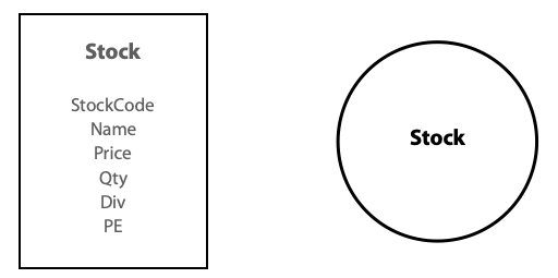
The Cypher code for creating a node for Stock is:
CREATE (:Stock {StockCode: "AR", Firm: "Abyssinian Ruby",
Price: 31.82, Qty: 22020, Div: 1.32, PE: 13});
Inserting nodes
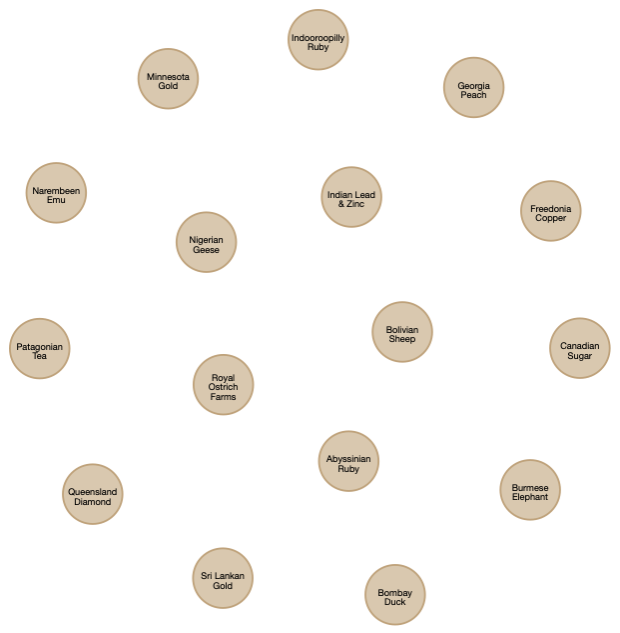
Usually, the data to populate a database exist in digital format, and if you can convert them to CSV format, such as an export of a spreadsheet, then you can use Cypher’s LOAD CSV command. The following code will create the nodes for each of the rows in a remote CSV file and return a count of how many nodes were created. You can load a local file by specifying a path rather than a url.
LOAD CSV WITH HEADERS FROM "https://www.richardtwatson.com/data/stock.csv" AS row
CREATE (s:Stock {StockCode: row.stkcode, Firm: row.stkfirm,
    Price: toFloat(row.stkprice), Qty: toInteger(row.stkqty), Div: toFloat(row.stkdiv),     PE: toInteger(row.stkpe)})
RETURN count(s);
The preceding code:
Specifies the url of the external CSV file with the temporary name row;
Creates a node with the label Stock and the temporary identifier s;
Reads a row at a time and converts the format, as appropriate, since all data are read as character strings. For example, toFloat(row.stkprice) AS Price reads a cell in the stkprice column on the input file, converts it to float format and associates it with the key Price to create a key:value pair for the node identified by StockCode.
When the preceding code is executed, it creates 16 unconnected nodes, as shown in the following figure.
Visualization of unrelated nodes in graph
Querying a node
This section mimics Chapter Three’s coverage of querying a single entity database. Many of the same queries are defined in Cypher code. As you should now have a clear idea of the results of a query, they are not shown in this chapter. You can alway run them with the Neo4j browser and look at the different forms of output it provides.
Displaying data for nodes with the same label
MATCH is Cypher’s equivalent of SELECT. A MATCH statement can report the properties for a particular type of node. Each node has an associated temporary identifier which is usually short (e.g., s). In this case, RETURN s, lists all the properties of Stock.
List all Stock data
MATCH (s:Stock)
RETURN s;
Reporting properties
The Cypher code for the equivalent of a relational project defines the keys of the properties to be displayed. Notice how a key is prefixed with the temporary name for the node (i.e., s) to fully identify it (e.g., s.Firm) and the use of AS to rename it for reporting (e.g., s.Firm AS Firm)
Report a firm’s name and price-earnings ratio.
MATCH (s:Stock)
RETURN s.Firm AS Firm, s.PE AS PE;
Reporting nodes
The Cypher code for the equivalent of a relational restrict also uses a WHERE clause to specify which nodes are reported. Neo4j supports the same arithmetic, Boolean, and comparison operators as SQL for use with WHERE.
Get all firms with a price-earnings ratio less than 12.
MATCH (s:Stock)
WHERE s.PE < 12
RETURN s;
Reporting properties and nodes
A single Cypher MATCH statement can specify which properties of which nodes to report.
List the name, price, quantity, and dividend of each firm where the share holding is at least 100,000.
MATCH (s:Stock)
WHERE s.Qty > 100000
RETURN s.Firm AS Firm, s.Price AS Price, s.Qty AS Quantity, s.Div AS Dividend;
IN for a list of values
As with SQL, the keyword IN is used with a list to specify a set of values.
Report data on firms with codes of FC, AR, or SLG.
MATCH (s:Stock)
WHERE s.StockCode IN ['FC','AR','SLG']
RETURN s;
❓ Skill builder
List those shares where the value of the holding exceeds one million.
Ordering rows
In Cypher, the ORDER BY clause sorts based on the value of one or more properties.
List all firms where the PE is at least 10, and order the report in descending PE. Where PE ratios are identical, list firms in alphabetical order.
MATCH (s:Stock)
WHERE s.PE >= 10
RETURN s
ORDER BY s.PE DESC, s.Firm;
Derived data
Calculations can be included in a query.
Get firm name, price, quantity, and firm yield.
MATCH (s:Stock)
RETURN s.Firm AS Firm, s.Price AS Price, s.Qty AS Quantity,
s.Div/s.Price*100 AS Yield;
Aggregate functions
Cypher has built-in functions similar to those of SQL, as the following two examples illustrate.
String handling
Cypher includes functions for string handling and supports regular expressions. The string functions are typical of those in other programming languages, such as toLower(), toUpper(), toString(), left(), right(), substring(), and replace(). For a complete list, see the Cypher manual.
Cypher supports regular expression using the syntax of Java’s regular expressions.
List the names of firms with a double ‘e’.
In the following code, the regular expression looks for any number of characters at the beginning or end of each string (.*) with two consecutive ’e’s ([e]{2}) in between.
Notice use of the toLower function to convert the firm name to all lower case so this query will work with any variation on consecutive ‘e’s, such as ’GEese’.
MATCH (s:Stock)
WHERE toLower(s.Firm) =~ '.*[e]{2}.*'
RETURN s.Firm;
You can also express the query using the Cypher CONTAINS clause, as follows:
MATCH (s:Stock)
WHERE s.Firm CONTAINS 'ee'
RETURN s.Firm;
Subqueries
A subquery requires you to determine the answer to another query before you can write the query of ultimate interest. The WITH clause chains subqueries by forwarding the results from one subquery to the next. For example, to list all shares with a PE ratio greater than the portfolio average, you first must find the average PE ratio for the portfolio, and then use the computed value in a second query.
Report all firms with a PE ratio greater than the average for the portfolio.
MATCH (s:Stock)
WITH AVG(s.PE) AS AvgPE
MATCH (s:Stock)
WHERE s.PE > AvgPE
RETURN s.Firm AS FIRM, s.PE as PE;
A relationship between nodes
We will use the data model in Chapter Four that records details of stocks listed in difference countries for illustrating a 1:m relationship between nodes. When developing a graph model, common nouns become labels (e.g., stock and country) and verbs become relationships. In the phrase “a nations lists many stocks,” we could extract the verb lists to use as a relationship name.
A graphical data model for an international portfolio of stocks
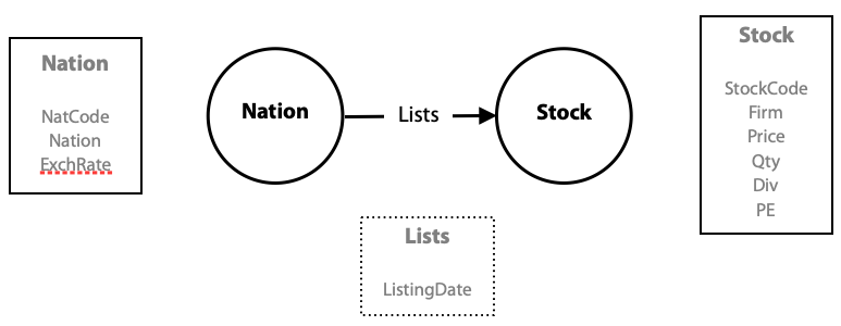
In this case, a country can list many stocks. First, we need to add four nation nodes to the graph database, as follows:
LOAD CSV WITH HEADERS FROM "https://www.richardtwatson.com/data/nation.csv" AS row
CREATE (n:Nation {NationCode: row.natcode, Nation: row.natname, ExchRate: toFloat(row.exchrate)})
RETURN count(n);
Specifying relationships in Cypher
Relationships are represented in Cypher using an arrow, either -> or <-, between two nodes. A node can have relationships to itself (i.e., recursive). In Neo4j, all relationships are directed (i.e., they are -> or <-).
The nature of the relationship is defined within square brackets, such as [:LISTS] in the case where a nation lists a stock on its exchange:
(n:Nation)-[:LISTS]->(s:Stock)If you want to refer to a relationship later in a query, you can define a temporary name. In the follow code sample, r is the temporary name for referring to the relationship LISTS.
MATCH (n:Nation)-[r:LISTS]->(s:Stock)Relationships can also have properties. The Cypher code for stating that Bombay Duck was listed in India on 2019-11-10 is:
MATCH (s:Stock), (n:Nation)
WHERE s.StockCode = "BD" AND n.NationCode = "IND"
CREATE (n)-[r:LISTS {Listed: date('2019-11-10')}]->(s)
RETURN r;
The WHERE clause specifies that nodes Bombay Duck and India are related. The third line of code creates the relationship by stating one nation, abbreviated as n, can list many stocks, abbreviated as s. The name of the relationship, LISTS, has the temporary name of r, which is is used in the RETURN r statement.
Rather than have to match each country and its listed shares as separate code chunks as with Bombay Duck, we can reread the stock file, stock.csv, because it has a column containing the nation code of the listing country. We match this code with a Nation node having the same value for nation code to create the relationship. In other words, the Cypher code creates the relationship by reading each row of stock.csv and matching its value for row.natcode with a Nation node that has the same value for the key NatCode. This is the same logic as matching a primary and foreign key to join two tables.
LOAD CSV WITH HEADERS FROM "https://www.richardtwatson.com/data/stock.csv" AS row
MATCH (n:Nation {NationCode: row.natcode})
MATCH (s:Stock {StockCode: row.stkcode})
CREATE (n)-[r:LISTS]->(s)
RETURN r;
Querying relationships
When defining relationship in a graph database, a programmer is effectively pre-specifying how two tables are joined. As a result, querying is slightly different from the relational style. Consider the following request:
Report the value of each stockholding in UK pounds. Sort the report by nation and firm.
The first step is define the relationship between the two nodes that contains the required properties to compute the value of the stockholding and then define the properties to be reported, the computation, and finally the sorting of the report.
MATCH (n:Nation)-[:LISTS]->(s:Stock)
RETURN n.Nation AS Nation, s.Firm AS Firm, s.Price AS Price, s.Qty as Quantity,
round(s.Price*s.Qty*n.ExchRate) AS Value
ORDER BY Nation, Firm;
WITH—reporting by groups
The WITH clause permits grouping nodes and it produces one row for each different value of the grouping node. The following example computes the value of the shareholding in UK pounds for each nation.
Report by nation the total value of stockholdings.
MATCH (n:Nation)-[:LISTS]->(s:Stock)
WITH n, round(sum(s.Price*s.Qty*n.ExchRate)) as Value
RETURN n.Nation AS Nation, Value;
Cypher’s built-in functions (COUNT, SUM, AVERAGE, MIN, and MAX) can be used similarly to their SQL partners. They are applied to a group of rows having the same value for a specified column.
Report the number of stocks and their total value by nation.
MATCH (n:Nation)-[:LISTS]->(s:Stock)
WITH n, count(s.StockCode) as Stocks, round(sum(s.Price*s.Qty*n.ExchRate)) as Value
RETURN n.Nation AS Nation, Stocks, Value;
❓ Skill builder
Report by nation the total value of dividends.
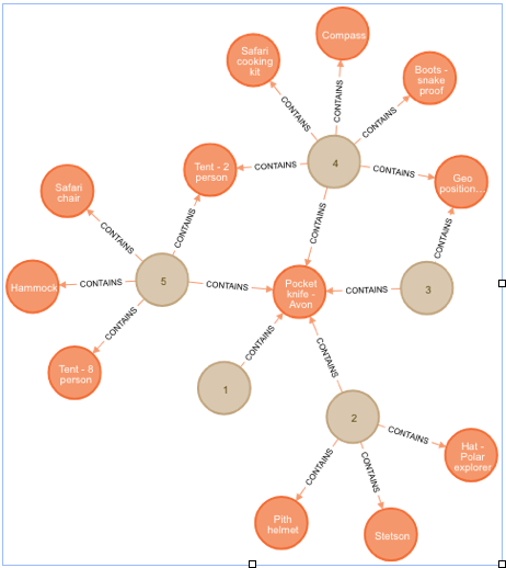
Querying an m:m relationship
In a graph database, a relationship replaces the associative entity used in a relationship model for representing an m:m. In the following graph model we could have indicated that an item can appear in many sales and a sale can have many items. For bidirectional relationships, ignore the direction when querying rather than create two relations.
A graph data model for sales
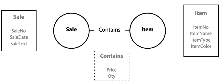
The sales example discussed in Chapter Five illustrates how to handle a many-to-many situation. We first load these data and then define the relationship. Notice that SET is used to establish the values of price and quantity properties of the relationship, which in a relational model are attributes of the associative entity. In practice, as each transaction occurs, an entry would be generated for each item sold.
LOAD CSV WITH HEADERS FROM "https://www.richardtwatson.com/data/item.csv" AS row
CREATE (i:Item {ItemNo: toInteger(row.itemno), ItemName: row.itemname, ItemType: row.itemtype, ItemColor: row.itemcolor})
RETURN count(i);

LOAD CSV WITH HEADERS FROM "https://www.richardtwatson.com/data/sale.csv" AS row
CREATE (s:Sale {SaleNo: toInteger(row.saleno), SaleDate: date(row.saledate), SaleText: row.saletext})
RETURN count(s);

LOAD CSV WITH HEADERS FROM "https://www.richardtwatson.com/data/receipt.csv" AS row
MATCH (s:Sale {SaleNo: toInteger(row.saleno)})
MATCH (i:Item {ItemNo: toInteger(row.itemno)})
CREATE (s)-[r:CONTAINS]->(i)
SET r.Price = toFloat(row.receiptprice), r.Qty = toInteger(row.receiptqty);
Once you have created the database, click on the CONTAINS relationship to get a visual of the database, as shown in the following figure. The nodes with numbers, SaleNo, are sales.
A view of the relationships between sales and items.
Here is an example of Cypher code for querying the graph for items and sales.
List the name, quantity, price, and value of items sold on January 16, 2011.
MATCH (s: Sale)-[r:CONTAINS]->(i: Item)
WHERE s.SaleDate = date(‘2011-01-16')
RETURN i.ItemName AS Item, r.Qty as Quantity, r.Price as Price, r.Qty*r.Price AS Total;
The preceding query could also be written as:
MATCH (s: Sale {SaleDate: date('2011-01-16')})-[r:CONTAINS]->(i: Item)
RETURN i.ItemName AS Item, r.Qty as Quantity, r.Price as Price, r.Qty*r.Price AS Total;
Does a relationship exist?
MATCH can be used to determine whether a particular relationship exists between two nodes by specifying the pattern of the sought relationship. The first query reports details of nodes satisfying a relationship.
Report all clothing items (type “C”) for which a sale is recorded.
MATCH (s: Sale)-[:CONTAINS]->(i:Item {ItemType: 'C'})
RETURN DISTINCT i.ItemName AS Item, i.ItemColor AS Color;
The second query reports details of nodes not satisfying a relationship.
Report all clothing items that have not been sold.
The query has a two stage process. First, identify all the items that have been sold and save their item numbers in SoldItems. Then, subtract this list from the the list of all items of type C to find the items not sold. This is similar to using a minus in SQL.
MATCH (s: Sale)-[:CONTAINS]->(i:Item {ItemType: 'C'})
WITH COLLECT (DISTINCT i.ItemNo) AS SoldItems
MATCH (i: Item)
WHERE i.ItemType = 'C' AND NOT (i.ItemNo IN SoldItems)
RETURN DISTINCT i.ItemName AS Item, i.ItemColor AS Color;
❓ Skill builder
Report all red items that have not been sold.
Recursive relationships
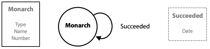
As you will recall, in data modeling a recursive relationship relates an entity to itself. It maps one instance in the entity to another instance of that entity. In graph terms, recursion relates nodes with the same label. The following diagram represents the previously discussed 1:1 monarch succession as graph.
A graph model for monarch
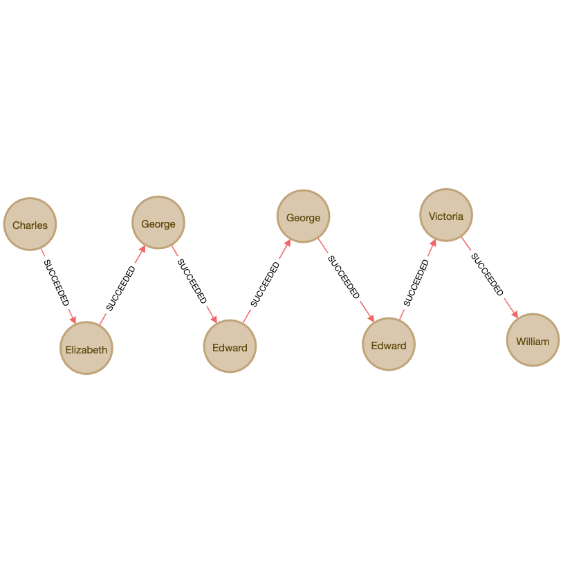
To assist with understanding the monarch model, we repeat the prior data.
Recent British monarchs
| Type | Name | Number | Reign begin |
|---|---|---|---|
| King | William | IV | 1830-06-26 |
| Queen | Victoria | I | 1837-06-20 |
| King | Edward | VII | 1901-01-22 |
| King | George | V | 1910-05-06 |
| King | Edward | VIII | 1936-01-20 |
| King | George | VI | 1936-12-11 |
| Queen | Elizabeth | II | 1952-02-06 |
| King | Charles | III | 2022-09-08 |
In the following Cypher code, observe the use of MATCH to connect each predecessor and successor monarch pair and the use of SET to define the succession date as a property of the succession relationship.
LOAD CSV WITH HEADERS FROM "https://www.richardtwatson.com/data/monarch.csv" AS row
CREATE (m: Monarch {Type: row.montype, Name: row.monname, Number: row.monnum})
RETURN count(m);

MATCH (p:Monarch), (s:Monarch) // p for predecessor and s for successor
WHERE p.Name = 'William' AND p.Number = 'IV' AND s.Name = 'Victoria' AND s.Number = 'I'
CREATE (s)-[r:SUCCEEDED]->(p)
SET r.Date = date('1837-06-20')
RETURN(r);

MATCH (p:Monarch), (s:Monarch)
WHERE p.Name = 'Victoria' AND p.Number = 'I' AND s.Name = 'Edward' AND s.Number = 'VII'
CREATE (s)-[r:SUCCEEDED]->(p)
SET r.Date = date('1901-01-22')
RETURN(r);

MATCH (p:Monarch), (s:Monarch)
WHERE p.Name = 'Edward' AND p.Number = 'VII' AND s.Name = 'George' AND s.Number = 'V'
CREATE (s)-[r:SUCCEEDED]->(p)
SET r.Date = date('1910-05-06')
RETURN(r);

MATCH (p:Monarch), (s:Monarch)
WHERE p.Name = 'George' AND p.Number = 'V' AND s.Name = 'Edward' AND s.Number = 'VIII'
CREATE (s)-[r:SUCCEEDED]->(p)
SET r.Date = date('1936-01-20')
RETURN(r);

MATCH (p:Monarch), (s:Monarch)
WHERE p.Name = 'Edward' AND p.Number = 'VIII' AND s.Name = 'George' AND s.Number = 'VI'
CREATE (s)-[r:SUCCEEDED]->(p)
SET r.Date = date('1936-12-11')
RETURN(r);

MATCH (p:Monarch), (s:Monarch)
WHERE p.Name = 'George' AND p.Number = 'VI' AND s.Name = 'Elizabeth' AND s.Number = 'II'
CREATE (s)-[r:SUCCEEDED]->(p)
SET r.Date = date('1952-02-06')
RETURN r;

MATCH (p:Monarch), (s:Monarch)
WHERE p.Name = 'Elizabeth' AND p.Number = 'II' AND s.Name = 'Charles' AND s.Number = 'III'
CREATE (s)-[r:SUCCEEDED]->(p)
SET r.Date = date('2022-09-08')
RETURN r;
The following figure shows the graph produced by Neo4j.
Monarch succession graph
Querying a recursive relationship
Some queries on the monarch graph database demonstrate the ease of querying a recursive relationship. Observe how to concatenate strings by using a plus (+) sign.
Who preceded Victoria I?
MATCH (s)-[r:SUCCEEDED]->(p)
WHERE s.Name = 'Victoria'
RETURN (p.Type + ' ' + p.Name + ' ' + p.Number);
Who succeeded Victoria I?
MATCH (s)-[r:SUCCEEDED]->(p)
WHERE p.Name = 'Victoria'
RETURN (s.Type + ' ' + s.Name + ' ' + s.Number);
List the kings and queens of England in ascending chronological order.
MATCH (s)-[r:SUCCEEDED]->(p)
RETURN (s.Type + ' ' + s.Name + ' ' + s.Number)
ORDER BY r.Date;
We see the power of a Cypher for querying a recursive relationship with the following query that uses *2 in the relationship pattern to select the second node in a chain of relationships.
Who was Elizabeth II’s predecessor’s predecessor?
MATCH (s)-[r:SUCCEEDED*2]->(p)
WHERE s.Name = 'Elizabeth' and s.Number = 'II'
RETURN (p.Type + ' ' + p.Name + ' ' + p.Number);
We can also select a series of nodes in a chain, and in the following example the first to third are selected by specifying *1..3 in the relationship pattern.
Who were Elizabeth II’s three immediate predecessors?
MATCH (s)-[r:SUCCEEDED*1..3]->(p)
WHERE s.Name = 'Elizabeth' and s.Number = 'II'
RETURN (p.Type + ' ' + p.Name + ' ' + p.Number);
The modeling and querying of 1:m and m:m recursive relationships are almost identical. Consider the case where an employee is the boss of other employees, then this could be expressed as:
MATCH (b:Employee), (e:Employee) // b for boss and e for employee
WHERE b.EmpCode = 1 AND e.EmpCode IN [2, 15, 23]
CREATE (b)-[r:IS_BOSS_OF]->(e);
and a query might start with:
MATCH (b)-[r:IS_BOSS_OF]->(e)For a recursive m:m, such as a bill of materials, we might write:
MATCH (a:Part), (p:Part) // a for assembly and p for part
WHERE a.PartCode = 1 AND p.PartCode IN [2,35,4,19,121]
CREATE (a)-[r:CONTAINS]->p;
Indexes and constraints
To speed up processing, indexes can be created on labels and property combinations. For example, the following code indexes the Stock label on the values of StockCode.
CREATE INDEX ON :Stock(StockCode);If you wanted to ensure all nation codes are unique, you would code:
CREATE CONSTRAINT ON (n:Nation) ASSERT n.NatCode IS UNIQUE;Remove duplicates
As with SQL, DISTINCT will remove duplicates from the results of a query.
MATCH (s:Stock)
RETURN DISTINCT s.PE AS PE;
Delete all nodes and relationships
To start afresh, use the following code to delete all nodes and relationships:
MATCH (a)
OPTIONAL MATCH (a)-[r]-()
DELETE a, r;
Conclusion
Graph databases are suitable for a wide range of common business problems. Graph analytics, in general, is useful for addressing three types of questions: How do things spread? What are the capacities, costs, and control points? How do things interact, and will that change?29
Summary
A labeled property graph database consists of nodes and relationships. Both nodes and relationships can have properties. A relationship is explicitly defined to connect a pair of nodes, and can have properties. Nodes and relationships can have properties in the form of key:value pairs. Nodes can be given one or more labels to group them. A graph description language (GDL) defines nodes and relationships. A graph query language (GQL) enables querying. Cypher is a GDL and GQL. A graph database is a good choice when many queries are about the network of relationships between nodes.
Key terms and concepts
| Edge | Node |
| Graph | Property |
| Label | Relationship |
References and additional resources
Francis, N., Green, A., Guagliardo, P., Libkin, L., Lindaaker, T., Marsault, V., . . . Taylor, A. (2018). Cypher: An evolving query language for property graphs. Paper presented at the Proceedings of the 2018 International Conference on Management of Data. https://dl.acm.org/doi/10.1145/3183713.3190657.
Robinson, I., Webber, J., & Eifrem, E. (2013). Graph databases: O’Reilly Media, Inc. ISBN: 1449356249
The following exercises are based on the Northwind graph database, which you can create on your computer by running the supplied code.
Graph model for Northwind
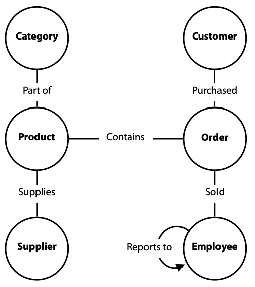
The Northwind database has the following relationships:
- (order)-[:CONTAINS]->(product)
- (employee)-[:SOLD]->(order)
- (customer)-[:PURCHASED]->(order)
- (supplier)-[:SUPPLIES]->(product)
- (product)-[:PART_OF]->(category)
- (employee)-[:REPORTS_TO]->(manager)
Exercises
Write Cypher code for the following queries.
How many employees are there in the company?
Prepare a list of employees by last name, first name, and job title. Sort by last name.
List the products that contain ‘sauce’ in their product description.
In what category are sauces?
List in alphabetical order those customers who have placed an order.
List in alphabetical order those customers who have not placed an order.
Which customers have purchased ‘Chai’?
List the amount ordered by each customer by the value of the order.
List the products in each category.
How many products in each category?
What is the minimum value of a received order?
Who is the customer who placed the minimum value order?
Report total value of orders for Blauer See Delikatessen.
Who reports to Andrew Fuller? Report by last name alphabetically and concatenate first and last names for each person.
Report those employees who have sold to Blauer See Delikatessen.
Report the total value of orders by year.
Basket of goods analysis: A common retail analytics task is to analyze each basket or order to learn what products are often purchased together. Report the names of products that appear in the same order three or more times.
ABC reporting: Compute the revenue generated by each customer based on their orders. Also, show each customer’s revenue as a percentage of total revenue. Sort by customer name.
Same as Last Year (SALY) analysis: Compute the ratio for each product of sales for 1997 versus 1996.
Needham, M., & Hodler, A. E. (2019). Graph Algorithms: Practical Examples in Apache Spark and Neo4j: O\’Reilly Media. ISBN: 1492047651↩︎