Chapter 18 Cluster computing
Let us change our traditional attitude to the construction of programs: Instead of imagining that our main task is to instruct a computer what to do, let us concentrate rather on explaining to humans what we want the computer to do
Donald E. Knuth, Literate Programming, 1984
Learning objectives
Students completing this chapter will:
Understand the paradigm shift in decision-oriented data processing;
Understand the principles of cluster computing
A paradigm shift
There is much talk of big data, and much of it is not very informative. Rather a lot of big talk but not much smart talk. Big data is not just about greater variety and volumes of data at higher velocity, which is certainly occurring. The more important issue is the paradigm shift in data processing so that large volumes of data can be handled in a timely manner to support decision making. The foundations of this new model is the shift to cluster computing, which means using large numbers of commodity processors for massively parallel computing.
We start by considering what is different between the old and new paradigms for decision data analysis. Note that we are not considering transaction processing, for which the relational model is a sound solution. Rather, we are interested in the processing of very large volumes of data at a time, and the relational model was not designed for this purpose. It is suited for handling transactions, which typically involve only a few records. The multidimensional database (MDDB) is the “old” approach for large datasets and cluster compute is the “new.”
Another difference is the way data are handled. The old approach is to store data on a high speed disk drive and load it into computer memory for processing. To speed up processing, the data might be moved to multiple computers to enable parallel processing and the results merged into a single file. Because data files are typically much larger than programs, moving data from disks to computers is time consuming. Also, high performance disk storage devices are expensive. The new method is to spread a large data file across multiple commodity computers, possibly using Hadoop Distributed File System (HDFS), and then send each computer a copy of the program to run in parallel. The results from the individual jobs are then merged. While data still need to be moved to be processed, they are moved across a high speed data channel within a computer rather than the lower speed cables of a storage network.
| Old | New |
|---|---|
| Data to the program | Program to the data |
| Mutable data | Immutable data |
| Special purpose hardware | Commodity hardware |
The drivers
Exploring the drivers promoting the paradigm shift is a good starting point for understanding this important change in data management. First, you will recall that you learned in Chapter 1 that decision making is the central organizational activity. Furthermore, because data-driven decision making increases organizational performance, many executives are now demanding data analytics to support their decision making.
Second, as we also explained in Chapter 1, there is a societal shift in dominant logic as we collectively recognize that we need to focus on reducing environmental degradation and carbon emissions. Service and sustainability dominant logics are both data intensive. Customer service decisions are increasingly based on the analysis of large volumes of operational and social data. Sustainability oriented decisions also require large volumes of operational data, which are combined with environmental data collected by massive sensor networks to support decision making that reduces an organization’s environmental impact.
Third, the world is in the midst of a massive data generating digital transformation. Large volumes of data are collected about the operation on an aircraft’s jet engines, how gamers play massively online games, how people interact in social media space, and the operation of cell phone networks, for example. The digital transformation of life and work is creating a bits and bytes tsunami.
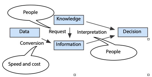
The bottleneck and its solution
In a highly connected and competitive world, speedy high quality decisions can be a competitive advantage. However, large data sets can take some time and expense to process, and so as more data are collected, there is a the danger that decision making will gradually slow down and its quality lowered. Data analytics becomes a bottleneck when the conversion of data to information is too slow. Second, decision quality is lowered when there is a dearth of skills for determining what data should be converted to information and interpreting the resulting conversion. We capture these problems in the elaboration of a diagram that was introduced in Chapter 1, which now illustrates the causes of the conversion, request, and interpretation bottlenecks.
Data analytics bottleneck
The people skills problem is being addressed by the many universities that have added graduate courses in data analytics. The Lambda Architecture46 is a proposed general solution to the speed and cost problem.
Lambda Architecture
We will now consider the three layers of the Lambda Architecture: batch, speed, and serving.
The batch layer
Batch computing describes the situation where a computer works on one or more large tasks with minimal interruption. Because early computers were highly expensive and businesses operated at a different tempo, batch computing was common in the early days of information systems. The efficiency gains of batch computing mainly come from uninterrupted sequential file processing. The computer spends less time waiting for data to be retrieved from disks, particularly with Hadoop where files are stored in 64Mb chunks. Batch computing is very efficient, though not timely, and the Lambda Architecture takes advantage of this efficiency.
The batch layer is used to precompute queries by running them with the most recent version of a dataset. The precomputed results are saved and can then be used as required. For example, a supermarket chain might want to know how often each pair of products appears in each shopper’s basket for each day for each store. These data might help it to set cross-promotional activities within a store (e.g., a joint special on steak and mashed potatoes). The batch program could precompute the count of joint sales for each pair of items for each day for each store in a given date range. This highly summarized data could then be used for queries about customers’ baskets (e.g., how many customers purchased both shrimp and grits in the last week in all Georgia stores?). The batch layer works with a dataset essentially consisting of every supermarket receipt because this is the record of a customer’s basket. This dataset is also stored by the batch layer. HDFS is well-suited for handling the batch layer, as you will see later, but it is not the only option.
New data are appended to the master dataset to preserve is immutability, so that it remains a complete record of transactions for a particular domain (e.g., all receipts). These incremental data are processed the next time the batch process is restarted.
The batch layer can be processing several batches simultaneously. It typically keeps recomputing batch views using the latest dataset every few hours or maybe overnight.
The serving layer
The serving layer processes views computed by the batch layer so they can be queried. Because the batch layer produces a flat file, the serving layer indexes it for random access. The serving layer also replaces the old batch output with the latest indexed batch view when it is received from the batch layer. In a typical Lambda Architecture system, there might be several or more hours between batch updates.
The combination of the batch and serving layers provides for efficient reporting, but it means that any queries on the files generated by the batch layer might be several or more hours old. We have efficiency but not timeliness, for which we need the speed layer.
Speed layer
Once a batch recompute has started running, all newly collected data cannot be part of the resulting batch report. The purpose of the speed layer is to process incremental data as they arrive so they can be merged with the latest batch data report to give current results. Because the speed layer modifies the results as each chunk of data (e.g., a transaction) is received, the merge of the batch and speed layer computations can be used to create real-time reports.
Merging speed and serving layer results to create a report (source: (Marz and Warren 2012))
Putting the layers together
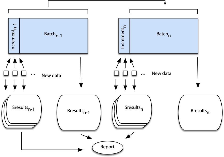
We now examine the process in detail.
Assume batchn-1 has just been processed.
During the processing of batchn-1, incrementn-1 was created from the records received. The combination of these two data sets creates batchn.
As the data for incrementn-1 were received, speed layer (Sresultsn-1) were dynamically recomputed.
A current report can be created by combining speed layer and batch layer results (i.e., Sresultsn-1 and Bresultsn-1).
Now, assume batch computation resumes with batchn.
Sresultsn are computed from the data collected (incrementn) while batchn is being processing.
Current reports are based on Bresultsn-1, Sresultsn-1, and Sresultsn.
At the end of processing batchn, Sresultsn-1 can be discarded because Bresultsn includes all the data from batchn-1 and incrementn-1.
The preparation of a real-time report using batch and speed layer results when processing batchn
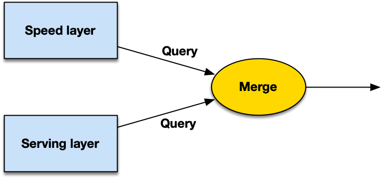
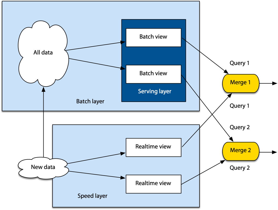
In summary, the batch layer pre-computes reports using all the currently available data. The serving layer indexes the results of the batch layers and creates views that are the foundation for rapid responses to queries. The speed layer does incremental updates as data are received. Queries are handled by merging data from the serving and speed layers.
Lambda Architecture (source: (Marz and Warren 2012))
Benefits of the Lambda Architecture
The Lambda Architecture provides some important advantages for processing large datasets, and these are now considered.
Robust and fault-tolerant
Programming for batch processing is relatively simple and also it can easily be restarted if there is a problem. Replication of the batch layer dataset across computers increases fault tolerance. If a block is unreadable, the batch processor can shift to the identical block on another node in the cluster. Also, the redundancy intrinsic to a distributed file system and distributed processors provides fault-tolerance.
The speed layer is the complex component of the Lambda Architecture. Because complexity is isolated to this layer, it does not impact other layers. In addition, since the speed layer produced temporary results, these can be discarded in the event of an error. Eventually the system will right itself when the batch layer produces a new set of results, though intermediate reports might be a little out of date.
Low latency reads and updates
The speed layer overcomes the long delays associated with batch processing. Real-time reporting is possible through the combination of batch and speed layer outputs.
Scalable
Scalability is achieved using a distributed file system and distributed processors. To scale, new computers with associated disk storage are added.
Support a wide variety of applications
The general architecture can support reporting for a wide variety of situations.
Extensible
New data types can be added to the master dataset or new master datasets created. Furthermore, new computations can be added to the batch and speed layers to create new views.
Ad hoc queries
On the fly queries can be run on the output of the batch layer provided the required data are available in a view.
Relational and Lambda Architectures
Relational technology supports both transaction processing and data analytics. As a result, it needs to be more complex than the Lambda Architecture. Separating out data analytics from transaction processing simplifies the supporting technology and makes it suitable for handling large volumes of data efficiently. Relational systems can continue to support transaction processing and, as a byproduct, produce data that are fed to Lambda Architecture based business analytics.
Hadoop
Hadoop, an Apache project, supports distributed processing of large data sets across a cluster of computers. A Hadoop cluster consists of many standard processors, nodes, with associated main memory and disks. They are connected by Ethernet or switches so they can pass data from node to node. Hadoop is highly scalable and reliable. It is a suitable technology for the batch layer of the Lambda architecture. Hadoop is a foundation for data analytics, machine learning, search ranking, email anti-spam, ad optimization, and other areas of applications which are constantly emerging.
A market analysis projects that the Hadoop market is growing at 48% per year.47 An early study48 asserts that, “Hadoop is the only cost-sensible and scalable open source alternative to commercially available Big Data management packages. It also becomes an integral part of almost any commercially available Big Data solution and de-facto industry standard for business intelligence (BI).”
Hadoop distributed file system (HDFS)
HDFS is a highly scalable, fault-toleration, distributed file system. When a file is uploaded to HDFS, it is split into fixed sized blocks of at least 64MB. Blocks are replicated across nodes to support parallel processing and provide fault tolerance. As the following diagram illustrates, an original file when written to HDFS is broken into multiple large blocks that are spread across multiple nodes. HDFS provides a set of functions for converting a file to and from HDFS format and handling HDFS.
Splitting of file across a HDFS cluster.
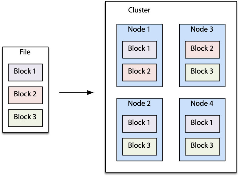
On each node, blocks are stored sequentially to minimize disk head movement. Blocks are grouped into files, and all files for a dataset are grouped into a single folder. As part of the simplification to support batch processing, there is no random access to records and new data are added as a new file.
Scalability is facilitated by the addition of new nodes, which means adding a few more pieces of inexpensive commodity hardware to the cluster. Appending new data as files on the cluster also supports scalability.
HDFS also supports partitioning of data into folders for processing at the folder level. For example, you might want all employment related data in a single folder.
Spark
Spark is an Apache project for cluster computing that was initiated at the University of California Berkeley and later transferred to Apache as an open source project. Spark’s distributed file system, resilient distributed dataset (RDD), has similar characteristics to HDFS. Spark can also interface with HDFS and other distributed file systems. For testing and development, Spark has a local mode, that can work with a local file system.
Spark includes several component, including Spark SQL for SQL-type queries, Spark streaming for real-time analysis of event data as it is received, and a machine learning (ML) library. This library is designed for in-memory processing and is approximately 10 times faster than disk-based equivalent approaches. Distributed graph processing is implemented using GraphX.
Computation with Spark
Spark applications can be written in Java, Scala, Python, and R. In our case, we will use sparklyr, an R interface to Spark. This package provides a simple, easy to use set of commands for exposing the distributed processing power of Spark to those familiar with R. In particular, it supports dplyr for data manipulation of Spark datasets and access to Sparks ML library.
Before starting with sparklyr, you need to check that you have latest version of Java on your machine. Use RStudio to install sparklyr. For developing and testing on your computer, install a local version of Spark.
Use the spark_connect function to connect to Spark either locally or
on a remote Spark cluster. The following code shows how to specify local
Spark connection (sc).
Tabulation
In this example, we have a list of average monthly temperatures for New York’s Central Park and we want to determine how often each particular temperature occurred.
Average monthly temperatures since 1869 are read, and temperature is rounded to an integer for the convenience of tabulation.
Spark example
By using dplyr in the prior R code, we can copy and paste and add a few commands for the Spark implementation. The major differences are the creation of a Spark connection (sc) and copying the R tibble to Spark with copy-to. Also, note that you need to sort the resulting tibble, which is not required in regular R.
library(dplyr)
library(readr)
spark_install(version='2.4')
sc <- spark_connect(master = "local", spark_home=spark_home_dir(version = '2.4'))
url <-  "http://www.richardtwatson.com/data/centralparktemps.txt"
t <- read_delim(url, delim=',')
t_tbl <- copy_to(sc,t)
t_tbl |>
  mutate(Fahrenheit = round(temperature,0)) |>
  group_by(Fahrenheit) |>
  summarize(Frequency = n()) |>
  arrange(Fahrenheit)
It you observe the two sets of output carefully, you will note that the results are not identical. It is because rounding can vary across systems. The IEEE Standard for Floating-Point Arithmetic IEEE 754 states on rounding, “if the number falls midway it is rounded to the nearest value with an even (zero) least significant bit.” Compare the results for round(12.5,0) and round(13.5,0). R follows the IEEE standard, but Spark apparently does not.
❓ Skill builder
Aedo the tabulation example with temperatures in Celsius.
Basic statistics with Spark
We now take the same temperature dataset and calculate mean, min, and max monthly average temperatures for each year and put the results in a single file.
Spark example
Again, the use of dplyr makes the conversion to Spark simple.
library(sparklyr)
library(tidyverse)
spark_install(version='2.4')
sc <- spark_connect(master = "local", spark_home=spark_home_dir(version = '2.4'))
url <-  "http://www.richardtwatson.com/data/centralparktemps.txt"
t <- read_delim(url, delim=',')
t_tbl <- copy_to(sc,t)
# report minimum, mean, and maximum by year
# note that sparkly gives a warning if you do not specify how to handle missing values
t_tbl |>
  group_by(year) |>
  summarize(Min=min(temperature, na.rm = T),
            Mean = round(mean(temperature, na.rm = T),1),
            Max = max(temperature, na.rm = T)) |>
  arrange(year)
❓ Skill builder
A [file][http://people.terry.uga.edu/rwatson/data/electricityprices2010_14.csv of electricity costs for a major city contains a timestamp and cost separated by a comma. Compute the minimum, mean, and maximum costs.
Summary
Big data is a paradigm shift to new file structures, such as HDFS and RDD, and algorithms for the parallel processing of large volumes of data. The new file structure approach is to spread a large data file across multiple commodity computers and then send each computer a copy of the program to run in parallel. The drivers of the transformation are the need for high quality data-driven decisions, a societal shift in dominant logic, and a digital transformation. The speed and cost of converting data to information is a critical bottleneck as is a dearth of skills for determining what data should be converted to information and interpreting the resulting conversion. The people skills problem is being addressed by universities’ graduate courses in data analytics. The Lambda Architecture, a solution for handling the speed and cost problem, consists of three layers: speed, serving, and batch. The batch layer is used to precompute queries by running them with the most recent version of the dataset. The serving layer processes views computed by the batch layer so they can be queried. The purpose of the speed layer is to process incremental data as they arrive so they can be merged with the latest batch data report to give current results. The Lambda Architecture provides some important advantages for processing large datasets. Relational systems can continue to support transaction processing and, as a byproduct, produce data that are fed to Lambda Architecture based business analytics.
Hadoop supports distributed processing of large data sets across a cluster of computers. A Hadoop cluster consists of many standard processors, nodes, with associated main memory and disks. HDFS is a highly scalable, fault-toleration, distributed file system. Spark is a distributed computing method for scalable and fault-tolerant cluster computation.
Exercises
Write Spark code for the following situations.
Compute the square and cube of the numbers in the range 1 to 25. Display the results in a data frame.
Using the average monthly temperatures for New York’s Central Park, compute the maximum, mean, and average temperature in Celsius for each month.
Using the average monthly temperatures for New York’s Central Park, compute the max, mean, and min for August. You will need to use subsetting, as discussed in this chapter.
Using the electricity price data, compute the average hourly cost.
Read the national GDP file, which records GDP in millions, and count how many countries have a GDP greater than or less than 10,000 million.
Marz, N., & Warren, J. (2012). Big Data: Manning Publications.↩︎